You have tried out Pivot Charts and have created one from an existing Pivot Table. Did you know that you can insert a pivot chart straight from the data source?
See how you can do this in just a couple of steps.
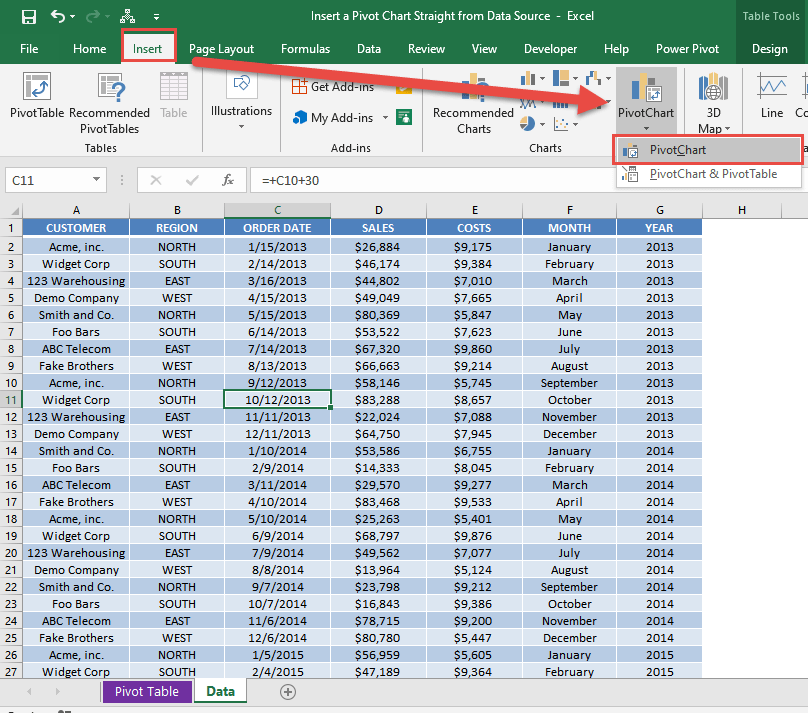
STEP 1: Select your data source. Go to Insert > Charts > PivotChart > PivotChart
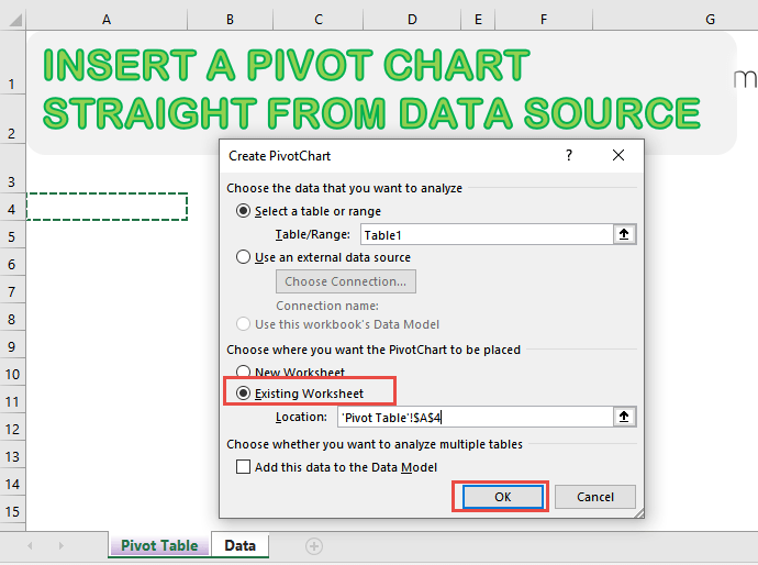
STEP 2: Select Existing Worksheet and pick a spot to place your Pivot Chart on. Click OK.
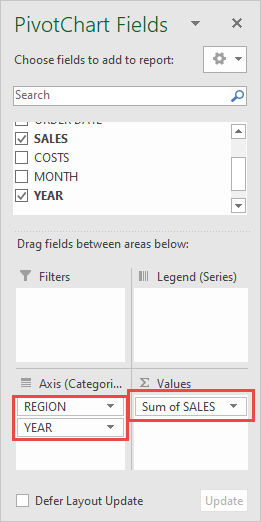
STEP 3: Let us quickly setup our Pivot Chart. Set the following:
Axis: Region and Year
Values: Sales
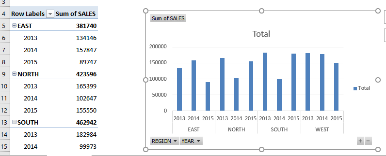
You now have your Pivot Chart straight from the data source!
How to Insert a Pivot Chart Straight From Data Source
Helpful Resource:

Bryan
Bryan Hong is an IT Software Developer for more than 10 years and has the following certifications: Microsoft Certified Professional Developer (MCPD): Web Developer, Microsoft Certified Technology Specialist (MCTS): Windows Applications, Microsoft Certified Systems Engineer (MCSE) and Microsoft Certified Systems Administrator (MCSA).
He is also an Amazon #1 bestselling author of 4 Microsoft Excel books and a teacher of Microsoft Excel & Office at the MyExecelOnline Academy Online Course.


