Pivot Tables allow you to analyze thousands of rows of data with just a few mouse clicks. It is the most powerful tool within Excel due to its speed and output and I will show you just how easy it is to create one.
If you are using a table or data set to analyze your information, then you should always use a Pivot Table which will enhance your analytical capabilities as well as save you heaps of time off your daily routine.
Pivot Tables are used by Project Managers, Finance Analysts, Auditors, Cost Controllers, Sales Analysts, Financial Controllers, Human Resources, Doctors and Statisticians just to name a few. Heck, I even created an in depth online course on Pivot Tables, that’s how in demand this Excel tool is in right at this moment!
Table of Contents
Insert a Pivot Table
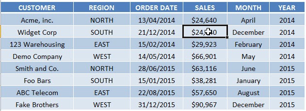
STEP 1: Click in your dataset. Make sure your data does not have any blank cells, columns or rows!
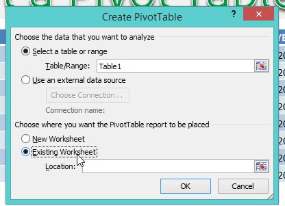
STEP 2: Go to Insert > Pivot Table
STEP 3: Place the Pivot Table in a New or Existing Worksheet
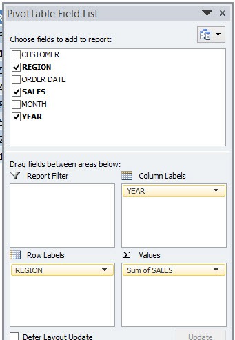
STEP 4: Drag and Drop the fields
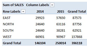
You now have your Pivot Table!
John Michaloudis is a former accountant and finance analyst at General Electric, a Microsoft MVP since 2020, an Amazon #1 bestselling author of 4 Microsoft Excel books and teacher of Microsoft Excel & Office over at his flagship MyExcelOnline Academy Online Course.


