How To Insert a Pivot Table Slicer
How To Insert a Pivot Table Slicer.
Slicers in Excel are visual filters or interactive buttons that allow you to see what items have been chosen within a Pivot Table.How To Insert a Pivot Table Slicer
Slicers in Excel are visual filters or interactive buttons that allow you to see what items have been chosen within a Pivot Table.
They are a new feature from Excel 2010 onward and Mac for Excel 2016 and a must for anyone wanting to wow their boss by adding interactivity in their reports! I show you how to insert a Pivot Table Slicer below:
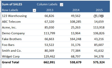
STEP 1: Select your Pivot Table by clicking anywhere inside it.
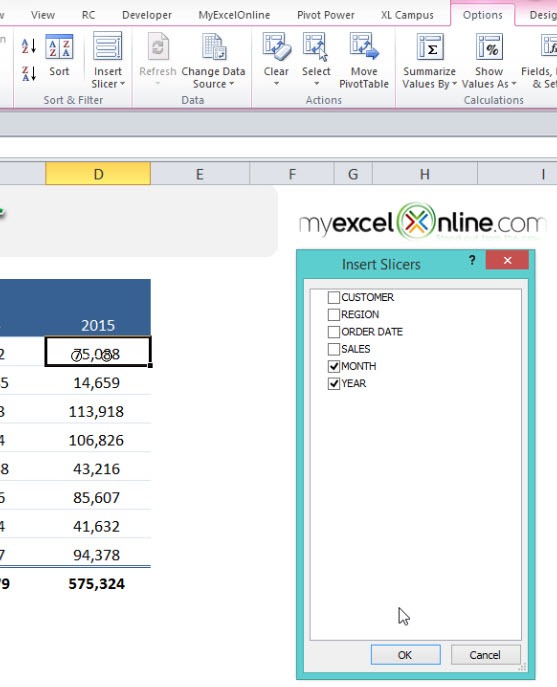
STEP 2: Go to Options(Excel 2010)/Analyze(Excel 2013&2016) > Insert Slicer
Select the Month and Year Fields.
Click OK.
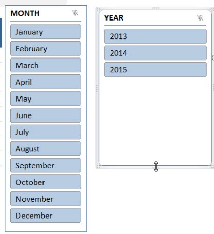
Your slicer is now ready! Go crazy clicking, slicing and dicing your data!
TIP: Hold down the CTRL key to select multiple items in your Slicer.
John Michaloudis is a former accountant and finance analyst at General Electric, a Microsoft MVP since 2020, an Amazon #1 bestselling author of 4 Microsoft Excel books and teacher of Microsoft Excel & Office over at his flagship MyExcelOnline Academy Online Course.


