Key Takeaways:
- Rounding numbers in Excel is crucial for simplifying data and ensuring consistency in analysis.
- The ROUND function is versatile, but I had to use a clever formula to round to the nearest multiple of 5.
- The MROUND function became my go-to for rounding to specific multiples, like 5, to maintain consistency across datasets.
- The CEILING and FLOOR functions helped me round numbers precisely up or down to the nearest multiple, which was essential for budgeting and pricing.
- Handling negative numbers and using special formats like ACCOUNTING in Excel made my data more accurate and professional.
Table of Contents
Getting Started with Excel Rounding Techniques
The Importance of Rounding Numbers in Excel
Rounding numbers in Excel simplifies complex data, making it more digestible for analysis and presentation. It helps in achieving consistency and clarity, especially when dealing with large data sets or presenting information to stakeholders who may not require detailed decimal precision.
By rounding, I ensure that the data remains an accurate representation of the original figures while being easier to work with.
Common Situations Where Rounding is Essential
We often encounter scenarios where rounding is vital. In financial reporting, it’s essential to present figures that are not only accurate but also readable; thus, revenue might be rounded to the nearest dollar. In inventory management, items may be grouped in multiples of five or ten for better bulk processing.
Similarly, when dealing with time tracking, hours worked might be rounded to the nearest quarter-hour for payroll calculations. These situations underscore how rounding directly impacts the clarity of data and the efficiency of decision-making processes.
The Basics of Rounding to the Nearest Multiple of 5
Understanding the ROUND Function
The ROUND function in Excel is fundamental for basic rounding. It is versatile, rounding to the nearest integer or to a specific decimal place depending on the need. This is incredibly useful when I’m preparing data that requires uniformity across figures or when I need to comply with specific numerical precision for reporting standards.
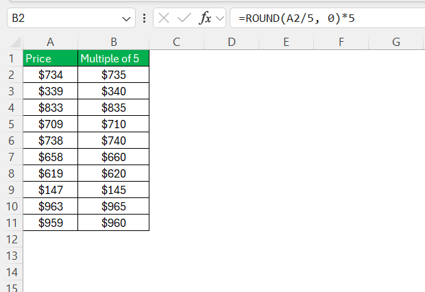
To utilize the ROUND function effectively for the nearest 5 or 50, a degree of ingenuity is needed since ROUND doesn’t directly allow for rounding to a specified multiple. If the goal is to round to the nearest 5, here’s the formula that does the trick: =ROUND(A2/5, 0)*5
.
This takes the original number, divides it by 5, rounds the result to the nearest whole number, and then multiplies it back by 5. It’s a neat math trick that leverages basic division and multiplication to create a custom rounding solution.
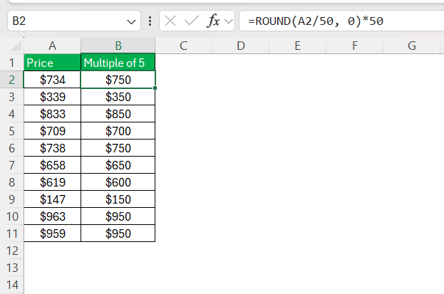
For rounding to the nearest 50, I simply replace 5 with 50 in the equation as follows: =ROUND(A2/50, 0)*50
.
This comes in handy when dealing with larger denominations or quantities, such as rounding off supply orders to the nearest box if each box contains 50 items.
By implementing such techniques, I ensure that my data sticks to predefined scales, whether for financial summarization, inventory packages, or when setting pricing strategies in multiple of 5 or 50. This rounding approach maintains the integrity of the numerical data while adhering to practical constraints.
How to Use the MROUND Function for Rounding to Multiples
To round off numbers to specific multiples in Excel, which is particularly useful when dealing with units that come in set quantities, I use the MROUND function. It rounds a given number to the nearest specified multiple.
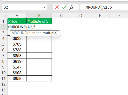
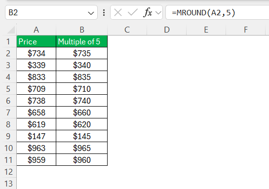
For example, if I need to round prices to the nearest nickel, I can use =MROUND(number, 5). This ensures that all prices are in increments that can actually be charged.
Here is how to use it:
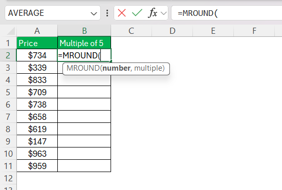
STEP 1: In a cell, type =MROUND(
.
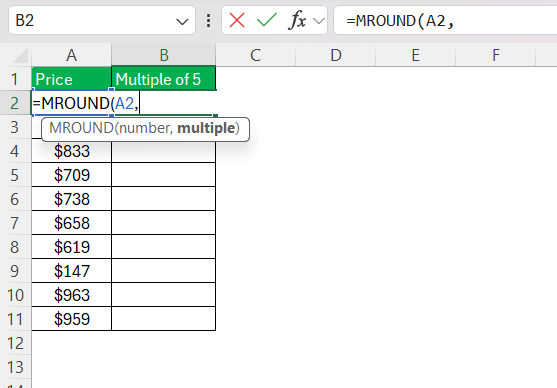
STEP 2: Enter the number to be rounded, followed by a comma.
STEP 3: Specify the desired multiple which the number should round to. Here, it is 5.
STEP 4: Close the parenthesis and hit enter.
This simple yet powerful function helps maintain consistency across datasets and is invaluable for logistical tasks like determining packaging sizes or planning transportation where goods are handled in multiples.
Advancing Your Skills: Complex Rounding Scenarios
Rounding with Precision Using CEILING and FLOOR Functions
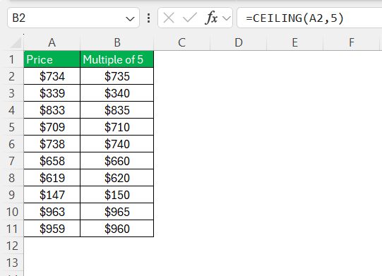
When I require precision in rounding, particularly for always rounding up or down to the nearest multiple, I turn to the CEILING and FLOOR functions in Excel. The CEILING function shines when I always want to round up to a specific multiple. This is useful for ensuring I never fall short, like in budgeting scenarios where rounding down could understate expenses.
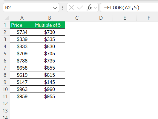
The FLOOR function, on the other hand, guarantees rounding down. For example, when I need to apply discounts or account for depreciation, I rely on it to etch down to the lower multiple, avoiding any overestimation.
To use CEILING:
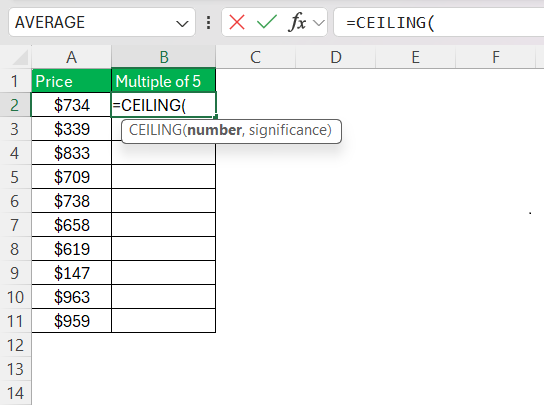
STEP 1: Input =CEILING(
in a cell.
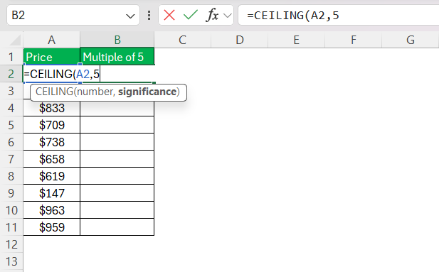
STEP 2: Follow this with the number, a comma, and the multiple to round up to.
STEP 3: Close the parenthesis and press enter.
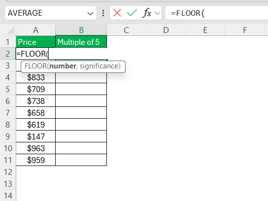
For FLOOR:
STEP 1: Start with =FLOOR(
.
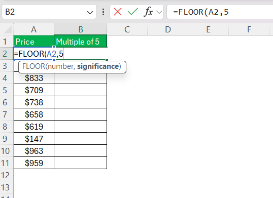
STEP 2: Input the number and the rounding multiple separated by a comma.
STEP 3: Close the parenthesis and hit enter.
These functions are indispensable tools in my Excel toolkit for scenarios like price setting or creating a floor or a cap on calculations that involve units of production or shipment sizes.
Tips for Handling Negative Numbers and Special Formats
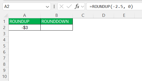
Handling negative numbers and special formats in Excel can be tricky, but with a few tips, I can navigate these challenges with ease. When working with negative numbers, it’s crucial to remember that functions like ROUNDUP and ROUNDDOWN handle them by first converting them to their absolute value, rounding accordingly, and then reapplying the negative sign.
For instance, using the ROUNDUP function on a negative number will actually decrease its value, even though it’s termed ‘up’. I keep in mind that ‘up’ refers to moving away from zero, so =ROUNDUP(-2.5, 0)
would give me -3.
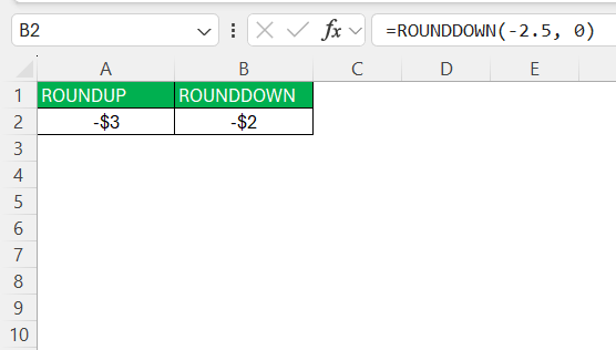
On the other hand, ROUNDDOWN tends to move closer to zero, so =ROUNDDOWN(-2.5, 0)
returns -2.
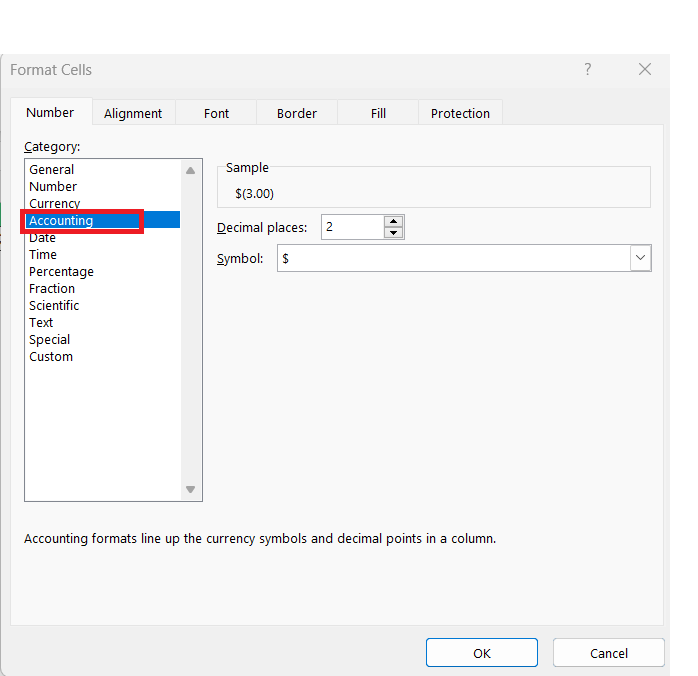
For special formats, like currencies, I use the ACCOUNTING format which nicely aligns decimal points and includes currency symbols. This is especially helpful for financial documents where clarity and uniformity are paramount. To apply this:
STEP 1: Click on the Home tab, and find the Number group.
STEP 2: Click the arrow next to the number formats and select ‘More Number Formats’.
STEP 3: Choose ‘Accounting’ and specify the number of decimal places.
These tips have saved me hours and ensured my spreadsheets are not only accurate but also presentable and professional.
FAQ: Navigating Common Rounding Queries
How do you multiply by 5 in Excel?
In Excel, to multiply a number by 5, I simply use the multiplication operator (*). For example, if I have a number in cell A1 that I want to multiply by 5, the formula would be =A1*5
. It’s a straightforward and quick way to scale any number by five in my spreadsheets.
How do I round to the nearest 5 in Excel?
To round to the nearest 5 in Excel, I use the MROUND function. The formula =MROUND(A1, 5)
rounds the number in cell A1 to the nearest multiple of 5. This function is handy for aligning figures with multiples that are commonly used for packaging, pricing, or operational thresholds.
What is the difference between ROUND, MROUND, CEILING, and FLOOR?
ROUND adjusts a number to a specified number of decimal places, MROUND rounds to the nearest specified multiple, CEILING always rounds up to the next multiple, and FLOOR always rounds down to the previous multiple. Each function serves a unique purpose for achieving different rounding results.
How can I ensure accuracy when rounding figures in financial reports?
To ensure accuracy when rounding figures in financial reports, I use the ROUND function to maintain consistency across all values. I’m also vigilant about using the same level of decimal precision throughout the report to prevent cumulative rounding errors, which is crucial for accurate totals and financial analysis.
How to get a multiple of a number in Excel?
To get a multiple of a number in Excel, I use the PRODUCT function or simple multiplication. For instance, =PRODUCT(A1, 5)
or =A1*5
gives me a result that is a multiple of 5 of the number in A1. It’s a simple and effective way to scale numbers by specific multiples.
John Michaloudis is a former accountant and finance analyst at General Electric, a Microsoft MVP since 2020, an Amazon #1 bestselling author of 4 Microsoft Excel books and teacher of Microsoft Excel & Office over at his flagship MyExcelOnline Academy Online Course.