Table of Contents
Pivot Table Number Formatting
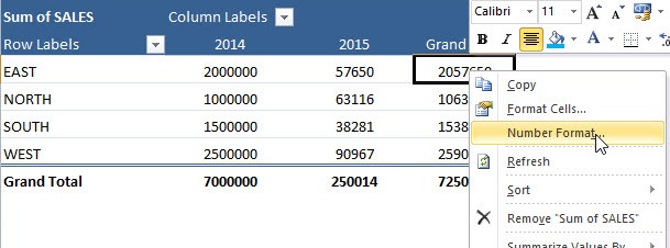
You can easily format your Pivot Table values simply by Right Clicking on a value and choosing Number Format. Then you can choose from the many different formats, like Number, Currency, Percentage or Custom.
STEP 1: Right click in the Pivot Table and choose Number Format
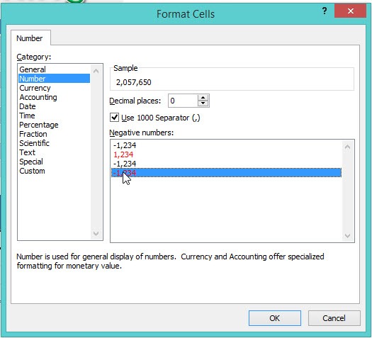
STEP 2: Choose your desired format
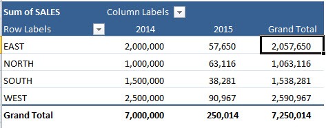
The Pivot table is now updated with your number formatting!
John Michaloudis is a former accountant and finance analyst at General Electric, a Microsoft MVP since 2020, an Amazon #1 bestselling author of 4 Microsoft Excel books and teacher of Microsoft Excel & Office over at his flagship MyExcelOnline Academy Online Course.


