How to Pull Information from Another Sheet Fast in Excel

I often find myself working with data spread across multiple worksheets within an Excel workbook. Whether I’m summarizing data, creating reports, or simply trying to consolidate information, knowing how to pull data from one worksheet into another is essential. In this article, we will cover different methods to pull information from another sheet in Excel.

Key Takeaways:

• Cell Referencing: Pull data from another worksheet by typing = in the target cell, selecting the desired cell from the source worksheet, and pressing Enter.
• Named Ranges: Use named ranges for easier formula management and clarity. Define a range name, then use it directly in your formulas.
• Lookup Functions: Use VLOOKUP for straightforward table lookups, and INDEX-MATCH for more flexible searches, especially when the lookup value isn’t in the first column.
• 3D Referencing: Consolidate data from multiple worksheets with 3D referencing by selecting a range of worksheets and using formulas like =SUM(‘2024:2026’!B2).
• Dynamic Data with Drop-Downs: Create drop-down lists using Data Validation and pull data based on the selection using the INDIRECT function, enabling dynamic data retrieval from different worksheets.

 

The Basics: Pull Information from Another Sheet

The most straightforward way to pull information from another worksheet is by directly referencing the cells. Here’s how I do it:

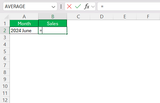
STEP 1: Start by typing an equal sign (=) in the cell where I want the data to appear. This tells Excel that I’m about to enter a formula.

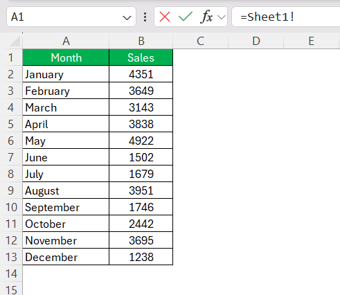
STEP 2: Navigate to the worksheet where the data is stored. I usually click on the worksheet tab at the bottom of the Excel window.

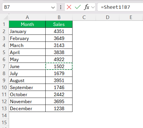
STEP 3: Click on the cell that contains the data I want to pull. Excel automatically inserts the worksheet name and the cell reference into the formula.

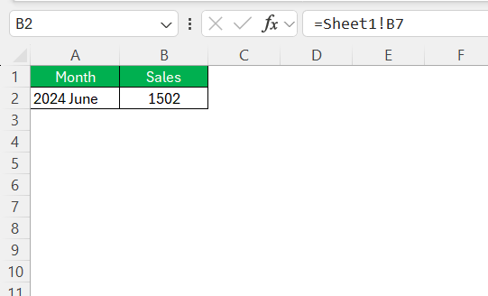
STEP 4: Press Enter to complete the formula. The data from the other worksheet now appears in the cell I started with.

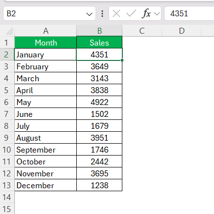
For example, if I’m on “Sheet2” and I want to pull data from cell B7 in “Sheet1,” my formula would look like this: =Sheet1!B7.

 

Using Named Ranges for Better Clarity

I like to use named ranges when I’m referencing specific areas in other worksheets. It makes the formulas easier to read and manage. Here’s how I do it:

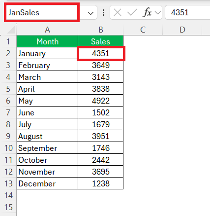
STEP 1: Select the range of cells I want to name in the source worksheet.

STEP 2: Click on the name box (to the left of the formula bar) and type a descriptive name, then press Enter. For example, I might name a range “JanSales”.

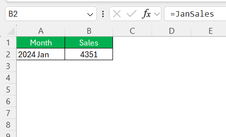
STEP 3: Use the named range in my formulas like this: =JanSales.

This way, I don’t have to worry about remembering specific cell references. Plus, it makes the formulas more intuitive.

 

Pulling Data Based on Criteria: Using VLOOKUP and INDEX-MATCH

Sometimes, I need to pull data based on specific criteria. That’s where functions like VLOOKUP and INDEX-MATCH come in handy.

VLOOKUP

I use VLOOKUP when I have a simple table where I need to find something in the first column and pull corresponding data from another column.

Here’s a quick example:

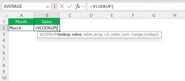
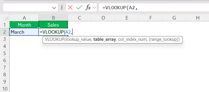
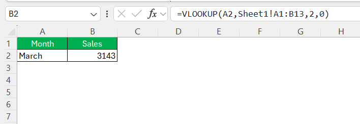
STEP 1: Type =VLOOKUP( in the cell where I want the data to appear.

STEP 2: Enter the lookup value (the value I’m searching for) followed by a comma. For example, =VLOOKUP(A2,.

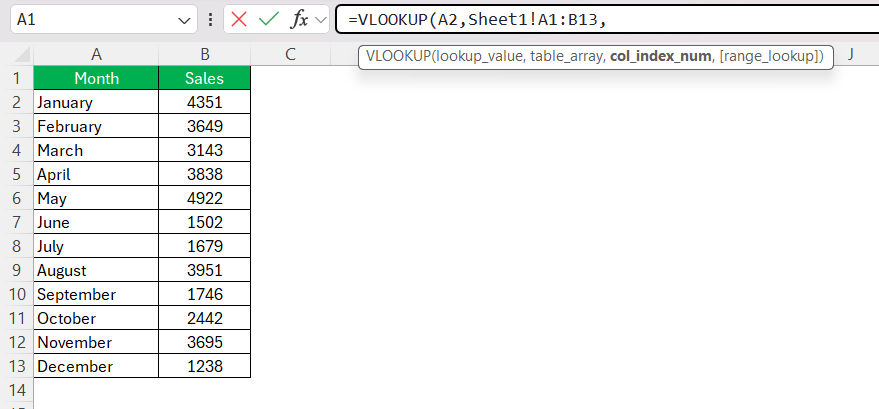
STEP 3: Select the range in the other worksheet where the data is located. I usually do this by clicking over to the other worksheet and dragging over the desired range.

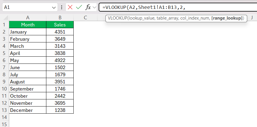
STEP 4: Specify the column index number (which column of the range contains the data I want to pull).

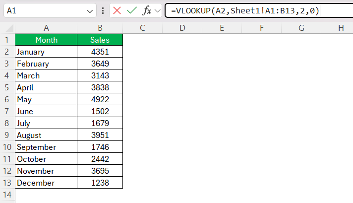
STEP 5: Enter 0 if I need an exact match, and close the parentheses. For example: =VLOOKUP(A2,Sheet1!A1:B13,2,0).

The result will be displayed.

INDEX-MATCH

I prefer using INDEX-MATCH when I need more flexibility than VLOOKUP offers, like when the lookup value isn’t in the first column.

Here’s how I do it:

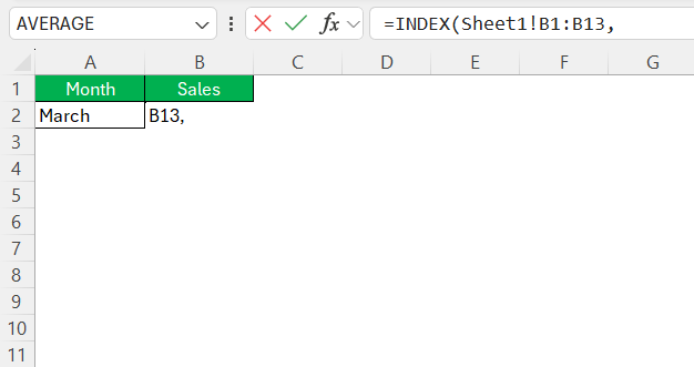
STEP 1: Type =INDEX( followed by the range that contains the data I want to return. For example, =INDEX(Sheet1!B1:B13,.

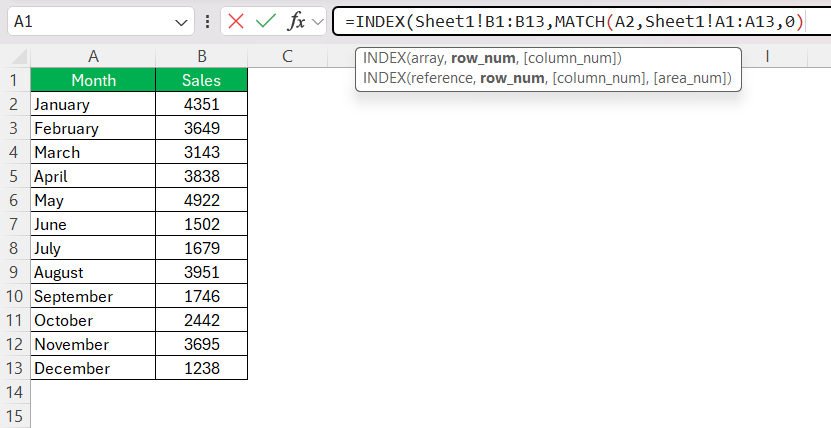
STEP 2: Type MATCH( followed by the lookup value and the range where I want to search for it, then close the MATCH function with a comma. For example: =INDEX(Sheet1!B1:B13,MATCH(A2,Sheet1!A1:A13,0)).

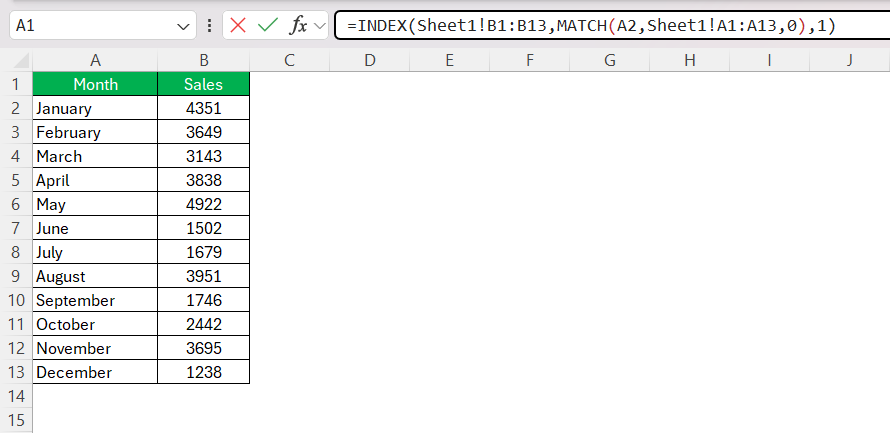
STEP 3: Close the INDEX function and press Enter.

This formula tells Excel to look for a value in a different worksheet, match it to a corresponding row, and return the data from a specific column.

Consolidating Data: 3D Referencing

Sometimes I have similar data across multiple worksheets that I want to consolidate. This is where 3D referencing comes into play.

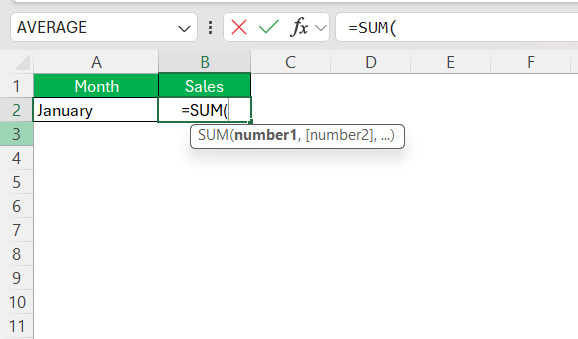
STEP 1: Start by typing a formula that you’d normally use, like =SUM(.

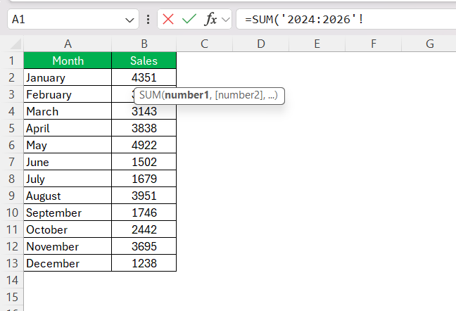
STEP 2: Select the range of worksheets that contain the data. I click on the first worksheet, hold Shift, and then click on the last worksheet.

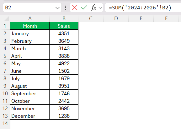
STEP 3: Select the cell range in the worksheet. Excel will automatically create a reference that includes all the worksheets.

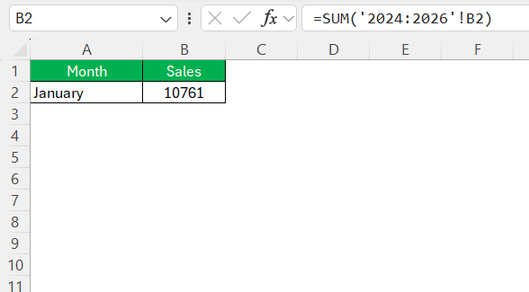
For example, to sum cell A1 across Sheets 2 to 4, I would use: =SUM('2024:2026'!B2).

 

Automating with Data Validation and Drop-Down Lists

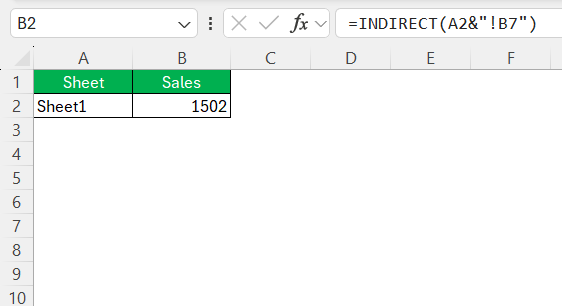
Sometimes I want to pull data from different worksheets based on a selection in a drop-down list. I use data validation to create the list and combine it with INDIRECT for the references.

• Create a drop-down list using Data Validation. I usually do this by selecting the cell, going to the Data tab, and choosing “Data Validation.”

• Set up the INDIRECT function to reference the selected value. For example: =INDIRECT(A2&"!B7") where A2 contains the worksheet name selected from the drop-down.

This way, I can dynamically pull information from different worksheets based on my selection

 

FAQ Section

How do I reference a cell from another worksheet in Excel?

To reference a cell from another worksheet, start by typing = in the desired cell, navigate to the worksheet with the data, and click on the cell you want to reference. Press Enter, and the data from that cell will appear in your current worksheet.

What is a named range, and how do I use it?

A named range is a descriptive label for a group of cells. To create one, select the cells, type a name into the name box, and press Enter. You can then use this name in your formulas instead of specific cell references, making your formulas easier to read and manage.

When should I use VLOOKUP versus INDEX-MATCH?

Use VLOOKUP when you need to find a value in the first column of a table and return data from another column. Use INDEX-MATCH for more flexibility, such as when the lookup value isn’t in the first column or when you need a more efficient lookup.

How can I consolidate data across multiple worksheets?

To consolidate data from similar cells across multiple worksheets, use a 3D reference. Start by typing a formula like =SUM(, select the range of worksheets, and then choose the cell range. Excel will sum the values from that cell across all selected worksheets.

Can I pull data from different worksheets based on a drop-down list?

Yes, you can use Data Validation to create a drop-down list and the INDIRECT function to reference the selected worksheet. This allows you to dynamically pull data based on your selection.