Numbers to Million Format: Quick Excel Format Guide

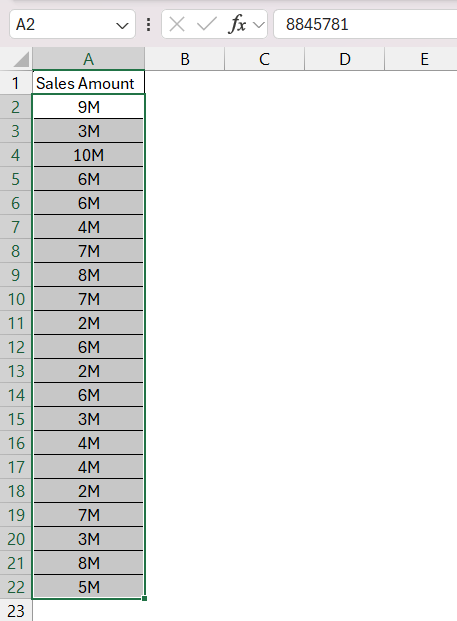
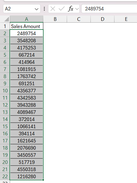
Microsoft Excel‘s number formatting is used for changing datasets into precise information. I will show you how you can convert large numbers into the Million format in just a couple of steps!

Key Takeaways

• Custom number formats in Excel let you control how numbers are displayed.
• You can use this formatting to make large numbers easier to read.
• Formatting numbers as millions improve readability and comparison, especially useful for financial and large-scale data.
• Conditional formatting with custom rules dynamically highlights significant data points, aiding in trend and outlier detection.

Download the spreadsheet and follow the blog on How to Convert to Million Format in Excel – Download excel workbookMillion-format-in-Excel.xlsx

Step-by-Step Guide for Million Format

Here’s a step-by-step guide to formatting your numbers as millions in Excel:

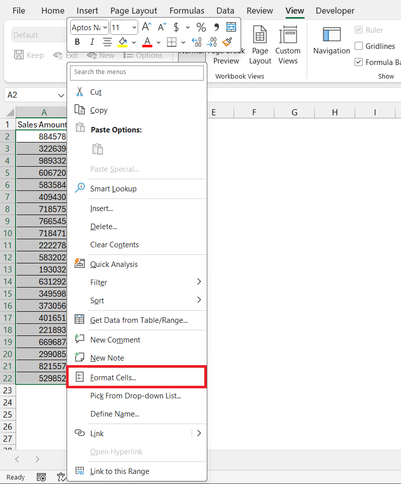
STEP 1: Right-click on the cell (or range of cells) that contains the number you want to format.

Select ‘Format Cells’ from the context menu to open the Format Cells dialog box.

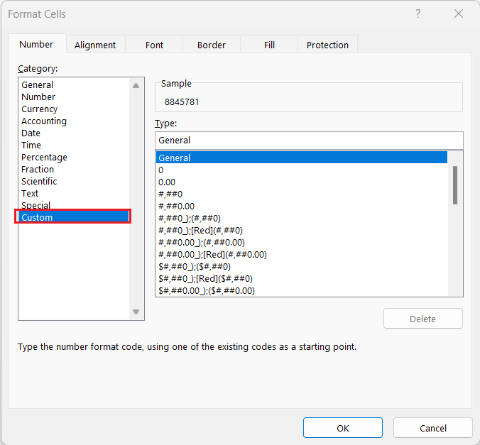
STEP 2: In the dialog box, go to Number > Custom 

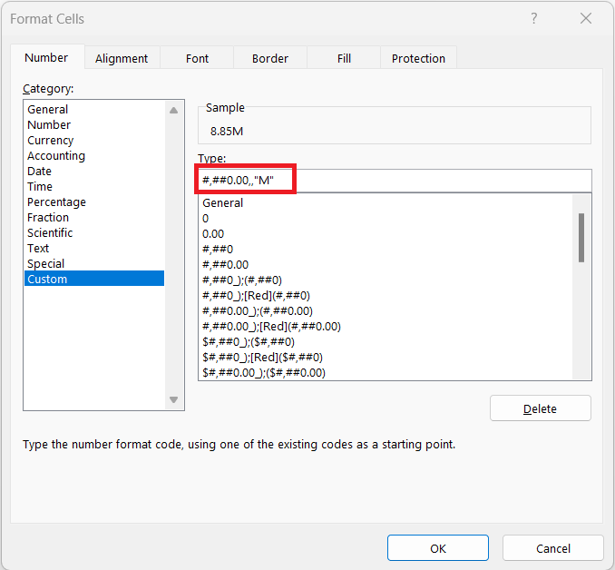
STEP 3: In the ‘Type’ input box, enter the format code: #,##0.00,,"M" for millions. This tells Excel to divide the number by a million and display two decimal places, followed by an “M” to indicate millions.

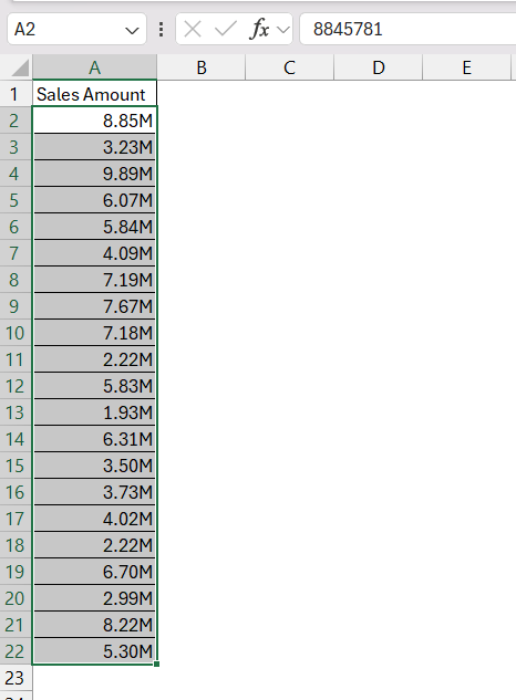
STEP 4: Click ‘OK’ to apply the custom format. Your numbers will now appear scaled to millions with the desired precision.

 

Rounding Large Numbers to Nearest Million Format

Sometimes, the specifics down to the last digit aren’t necessary, and a rounded figure can better fit your needs. In Excel, you can round large numbers to the nearest million.

For rounding numbers to the nearest million in Excel:

STEP 1: Click on the cell you want to format. Right-click and select ‘Format Cells’ from the context menu.

STEP 2: On the Number tab, select ‘Custom’.

STEP 3: Enter the format code #,##0,,"M" into the Type box. This code rounds your numbers to the nearest million and appends an “M” to signify the million format.

STEP 4: Hit ‘OK’ to see your numbers rounded off.

While rounding provides a cleaner look, it’s best used when exact values are not crucial to your analysis.

 

Advanced Tips

Using Conditional Formatting with Custom Rules

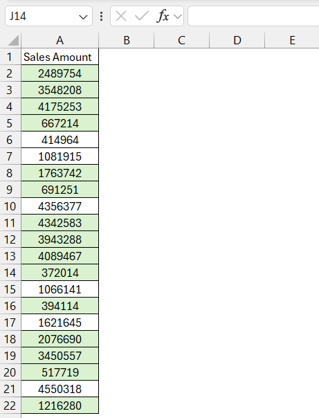
You can also use conditional formatting with custom rules. See this example below:

STEP 1: Select the range of cells you want to format.

STEP 2: Navigate to the ‘Home’ tab, click on ‘Conditional Formatting’, and choose ‘New Rule’.

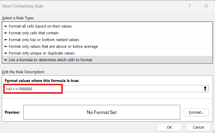
STEP 3: Select ‘Use a formula to determine which cells to format’. Create a formula based on your conditions—let’s say, to format cells greater than a million, you’d use: =A1>=1000000.

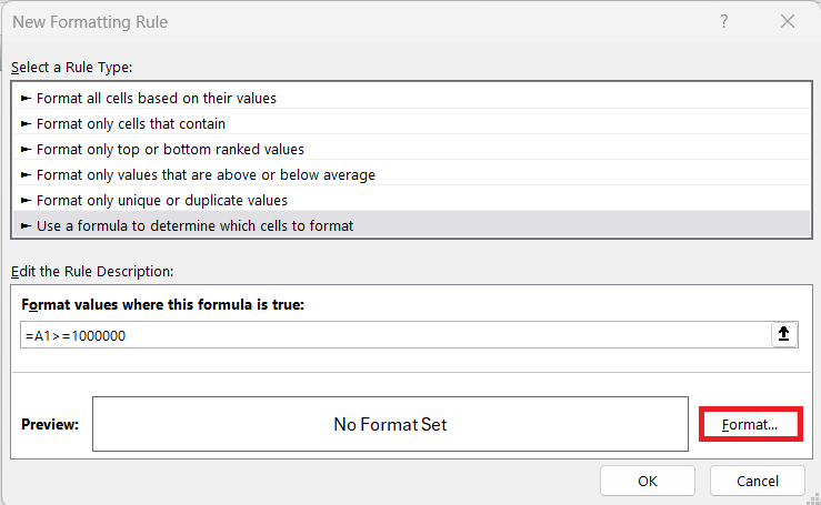
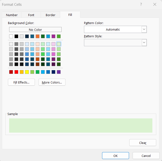
STEP 4: Then, set the desired format by clicking ‘Format’.

STEP 5: Press ‘OK’ twice to apply the rule.

This highlights values above a certain threshold with conditional formatting.

 

FAQs on Excel Millions Format

How Do I Convert Numbers to Show as ‘1M’ Instead of ‘1,000,000’?

To display ‘1M’ instead of ‘1,000,000’, select your cell or range, then press [Ctrl] + 1 to open the Format Cells dialog. Under Custom, type #,##0,,"M" and hit OK.

Does this also work for negative numbers?

Yes, you can use custom formatting to change how negative numbers appear in Excel. Create a format with a second section for negatives like 0;[Red]-0 to make negatives red.

For parentheses, use 0;[Red](0).  Apply this by right-clicking the cell, selecting ‘Format Cells’, and typing your code in ‘Custom’.

Can I Add Currency Symbols While Formatting to Millions?

Yes, to add currency symbols while formatting to millions, follow the custom format structure by including the currency symbol directly in the format code.

For example, for US dollars, you may use "$#,##0.00,,"M".  This combines the currency format with the million indicators, neatly displaying the values as, for instance, “$1.00M”.

How do you format data labels to millions in Excel?

To format data labels to millions in Excel charts, right-click on a data label, then click ‘Format Data Labels’.

In the pane, select ‘Number’, and under ‘Custom’, input the code 0.0,,"M".

Press ‘Add’ and the labels will display in millions, such as “1.5M” for 1,500,000.