Excel Custom Number Format Millions and Thousands

The Power of Custom Formatting

Imagine having a magic wand to make your Excel data tell the story you want it to. The power of custom formatting in Excel is just like that wand. With a few clicks, I was able to twist and turn my numbers to display in a format that’s more than just digits. It’s about presenting them in ways that immediately highlight what’s important, whether it’s breaking down sales targets, budget forecasts, or project timelines.

Many times, I have large numbers in an Excel report and it is hard to decipher and read the number at one glace.

The best way is to show the numbers in Thousands (K) or Millions (M).

Say, a number 45,200,000 will be displayed as 45.2 Million. This is what I did:

Key Takeaways

• Excel allows users to condense large numerical datasets into more readable formats by using custom number formatting to represent numbers in terms of “thousands (K),” “millions (M),” or “billions (B).”
• To format numbers into thousands or millions in Excel, select the cells to be formatted, press Ctrl + 1 to open the Format Cells window, switch to the Custom option and enter the appropriate code (e.g., 0,”Thousands” for thousands; the exact code can vary).
• Utilizing the custom number formatting feature in Excel simplifies data presentation and analysis, helping users to quickly comprehend figures that would otherwise be lengthy and cumbersome to read in their full numerical form.

Custom Formatting

Fortunately, large numbers in Excel can be formatted so they can be shown in “Thousands” or “Millions”.

By using the Format Cells dialogue box shortcuts CTRL+1, you will need to select CUSTOM and then enter one comma to show Thousands or two commas to show Millions. You can even add some text in your cells by entering any word within the quotation marks ” your word “.

But before we move forward, it is important to know that certain characters in custom formatting have specific meaning.

• Zero (0) – Display insignificant zeros
• Pound Sign (#) – Display significant zeros
• Comma (,) – Thousand separator
• Quote (” “) – Add text present within the quotes

You can create Excel Custom Number Format Millions and Thousands using either placeholder zero or pound sign. Let’s look at both of them one-by-one.

 

With Placeholder Pound Sign (#)

#,##0, “ths”

#,##0,, “mills”

In the example below, you have sales data with the sales amount mentioned in columns D & E. Using the Excel number formatting, you need to convert excel format number in millions & thousands.

 

 

Follow the step-by-step tutorial to understand how to add Excel custom number format millions and thousands and make sure to download this workbook to follow along:

Download workbookNumber-Formats-Ths-Mills.xlsx

 

STEP 1: Select Column D in the data below.

 

STEP 2: Press Ctrl + 1 to open the Format Cells dialog box.

 

STEP 3: In the Format Cells dialog box, Under Number Tab select Custom.

 

STEP 4: Type #,##0, “ths” and Click OK.

 

STEP 5: This is how the Column D after number formatting will look –

 

STEP 6: Follow the same steps for Column E as well and type #,##0,, “mills” under the custom section.

The only difference between the two customer format (Thousands & Millions)  is that you have to put 1 comma for Thousands and two commas for Millions.

 

Using Placeholder Zero (0) & Decimal Point

0.0, “K”

0.0,, “M”

 

Zero is used to display insignificant zeros when the number has fewer digits than the format represented using zero. For example, a custom format 0.00 will display number 5, 8.5, and 10.99 as 5.00, 8.50, and 10.99 respectively.

Also, you can round off the number using decimal points symbol.

 

To get this formatting done, follow the steps below:

STEP 1: Select Column D in the data below.

 

STEP 2: Right-Click and then Select Format Cells.

 

STEP 3: In the Format Cells dialog box, Under Number Tab select Custom.

 

STEP 4: In the Type section, type format – 0.0, “K” and click OK.

Follow the same process for formatting Numbers in Millions.

 

STEP 5: In the type section, Enter 0.0,, “M” and Click OK.

Excel number format millions & thousands is now ready!

One thing to note is that this will just format the way the number looks like on the Sheet. The number stored in the cell remains the same!

You can use the ROUND function to not just change the formatting but the change the number as well.

 

ROUND Function

In this method, you have to do three things :

• Divide the number by 1000,000.
• Round off the decimal places.
• Use & sign to add text “M”.

 

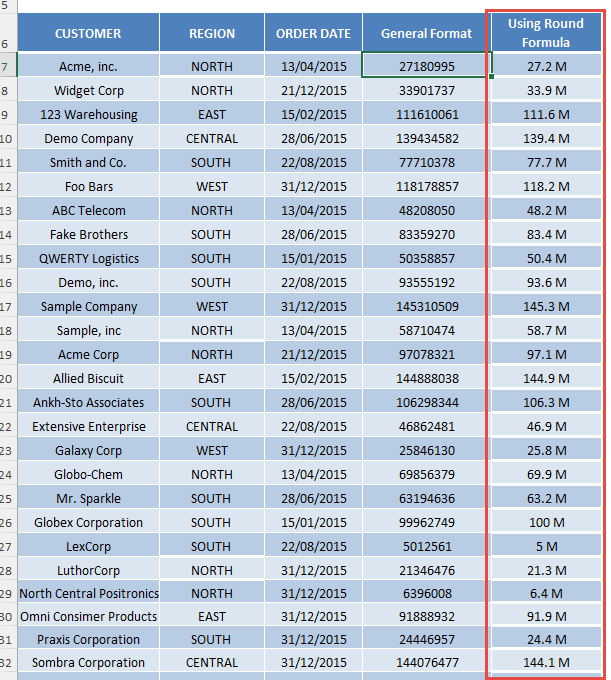
In this example, you have the sales amount mentioned in Column D. Let’s use the combination of division, round, and & sign to get the formatting done.

 

STEP 1: Select cell E7.

 

STEP 2: Start with the division. Type =D7/1000000.

 

STEP 3: Add Round Function to this. Type =ROUND(D7/1000000,1).

 

STEP 4: Add Text to this formula using & sign. Type =ROUND(D7/1000000,1)&” M”.

 

STEP 5: Copy the formula down.

 

STEP 6: Copy the Column and the Press Alt + E + S to open the Paste Special Box and Select Value. Click OK.

 

The only difference between using Custom Format & Round Function is that :

• In Custom Format, only the formatting changes but the number stored remains the same.

• In Round Function, both the formatting and number changes.

 

Advanced Excel Tricks for Perfect Formatting

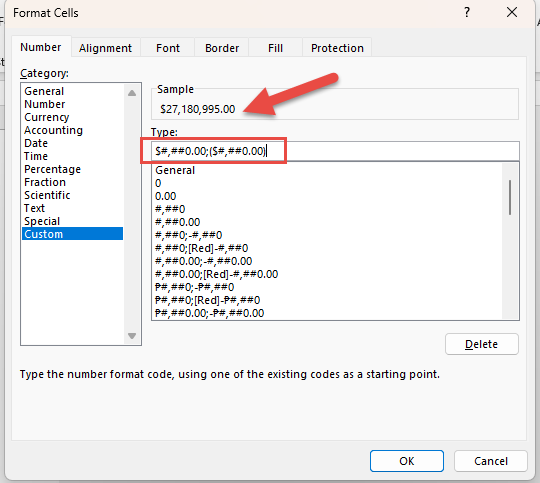
Incorporating Currency Symbols for Financial Figures

When dealing with financial figures, getting the currency right is as important as the numbers themselves. In Excel, incorporating currency symbols into your data is straightforward. If you’re working with dollars, simply use $ in your custom number format—like $#,##0.00;($#,##0.00) to show positive numbers and embrace negative ones with parentheses. For other currencies, you might need a helping hand from ANSI codes—for example, ALT+0128 for Euro (€). Add these symbols directly in the format code section, and watch as your numbers transform into meaningful financial data.

Dealing with Decimals and Negative Numbers Gracefully

Navigating decimals and negative numbers with grace ensures that your Excel sheets remain clear and understandable, no matter the complexity. To handle decimals, decide how many places are significant for your data and use a format like 0.00 to always show two decimal places, or #,##0.## to display them only when they exist. For negative numbers, choose a format that highlights them, such as (#,##0), which wraps negatives in parentheses, or #,##0;-#,##0 to show them in red. These tweaks maintain readability and instantly draw the eye to crucial figures that might need attention.

Real-life Applications of Custom Number Formats

Making Financial Statements More Readable

Financial statements carry the weight of business insights, and their readability can make or break decision-making processes. Custom number formatting in Excel streamlines figures and highlights the critical financial health indicators. Say goodbye to eye-straining lists of digits and welcome clean, rounded numbers that executives can comprehend at a glance. By using formats that abbreviate to thousands or millions and maintaining a consistent layout, your financial statements not only look professional but become far more user-friendly.

You could see the highlighted column below as a lot easier to read and digest:

Fine-tuning Reports for Better Stakeholder Communication

Fine-tuning reports goes beyond number crunching; it’s about tailoring data presentation for stakeholder communication. Through strategic use of custom number formats, you can highlight what’s vital and convey the right message without overwhelming your audience with data. Whether it’s summing up annual expenditures or showcasing quarterly profits, the numbers on your reports should speak to stakeholders clearly. With Excel, the goal is to make every digit informative and every figure a potential conversation starter.

Common Pitfalls and How to Avoid Them

Ensuring Compatibility Across Various Excel Versions

Ensuring that your custom number formats work seamlessly across different Excel versions is crucial for maintaining data integrity. Be mindful that some formats may not translate perfectly if you’re sharing files between the latest Excel version and older ones. To avoid hiccups, stick with universal formatting options and avoid using features exclusive to newer releases when you know the file will be opened in earlier versions. Test your spreadsheets in various environments to confirm their resilience and ensure that your formatting enchantments don’t lose their power when shared across different versions of Excel.

FAQs on Mastering Excel’s Number Formatting

How do you format thousands and million in Excel?

To format numbers as thousands or millions in Excel, select the cells to format and press Ctrl + 1 to open the Format Cells dialog. Then choose ‘Custom’ and type 0,"K" to format as thousands or 0,,"M" to format as millions. This will transform your numbers into a more digestible format by showing just the amount in thousands or millions, rather than the full number.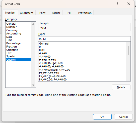

Can You Round Numbers to the Nearest Thousand in Excel?

Absolutely, you can round numbers to the nearest thousand in Excel using the ROUND function. Simply type =ROUND(your_number,-3) in a cell next to the one you want to round. This formula takes the number in your specified cell and rounds it to the nearest thousand, making your data much easier to work with, especially when dealing with large numbers.

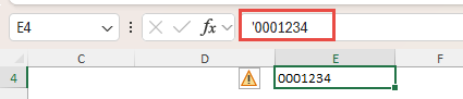
How Do You Maintain Leading Zeros When Formatting?

To keep leading zeros in Excel, start by selecting the cell or range where you want the zeros maintained. Then, right-click and choose ‘Format Cells.’ Under the ‘Number’ tab, select ‘Text’ to treat your entry as text or prepend your number with an apostrophe (‘), like so: '0001234. This signals Excel to preserve the zeros as they are without converting the value to a number.

What’s the Difference Between Using Comma and Period in Number Formats?

In number formats, the comma typically serves as a thousands separator, helping break up large numbers for easy reading, while the period is used as a decimal point to separate whole numbers from fractional parts. However, this can vary based on regional settings where some countries use a period for thousands and a comma for decimals. Always ensure you’re using the correct format for your audience’s locale to avoid confusion.

Is There a Way to Apply Conditional Number Formatting Based on Cell Value?

Yes, Excel allows for conditional number formatting based on a cell’s value. Use the ‘Conditional Formatting’ feature found on the Home tab. With it, you can set rules using comparison operators like greater than, less than, or equal to, with custom formats that apply only if the condition is met. For example, [Red][<10];[Green][>=10] turns numbers less than 10 red and those greater or equal to 10 green.

Conclusion

In this article, you have been taught how to do Excel custom number format millions and thousands. There are two ways to do so. You can either use custom format options available in Excel or use a combination of division, round, and & sign.

There are various analytical tools inside Excel, like Conditional Formatting, Data Validation, Tables, Sort & Filter plus MORE!  Click here to learn more!

You can learn more about Excel with Formulas, Pivot Tables, and Macros here!