Conditional Formatting A Drop Down List

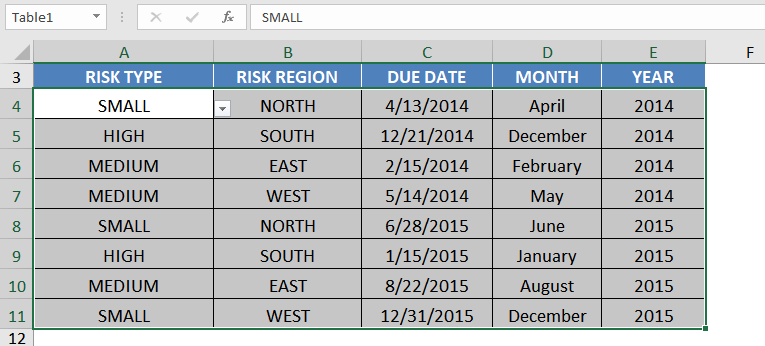
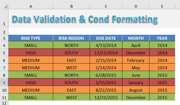
In a previous post I showed you how to Create a Drop Down List in a Table.   We are now going to take this concept one level further and apply some conditional formatting to the drop down data validation list. This is useful if you want to highlight when a job is completed, check off items from a list or to evaluate risk in a project just like I have done in the example below.

Key Takeaways

• Conditional formatting in dropdown lists serves as a beneficial tool in Excel to visually communicate the status of tasks or items, such as indicating a completed job or evaluating project risks. By changing cell colors based on selected items, users can quickly grasp task progress or data and make spreadsheets more efficient and user-friendly.
• Implementing conditional formatting to dropdown lists not only enhances the presentation of data but also aids in preventing incorrect data entries by guiding users to select from predefined options instead of manually typing, leading to more accurate and reliable data input.
• Adding conditional formatting to dropdown lists can be a powerful feature for those handling assignments or projects in school or at the workplace, providing a simple yet effective way to make data stand out, save time for users, and impress audiences with clear and visually appealing spreadsheets.

Want to know all about Conditional Formatting from Beginner to Advanced?

*** Watch our video and step by step guide below with free downloadable Excel workbook to practice ***

Watch it on YouTube and give it a thumbs-up!

STEP 1: Select the range that you want to apply the conditional formatting to.

 

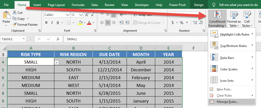
STEP 2: Go to Home > Styles > Conditional Formatting > Manage Rules

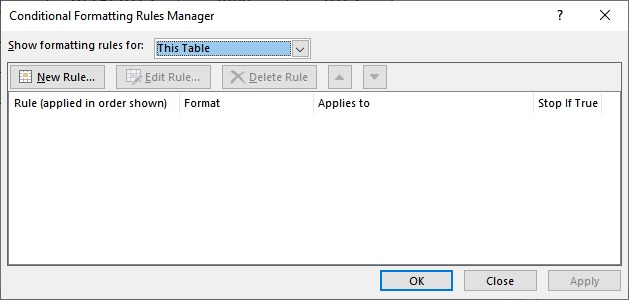
STEP 3: Select New Rule

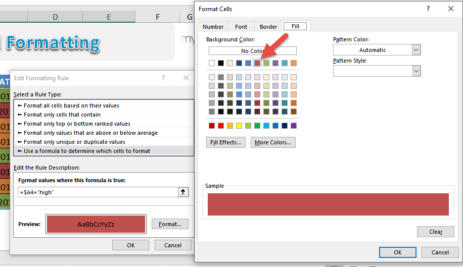
STEP 4: Create the new rule for High values:

Select Use a formula to determine which cells to format

Type in the Formula =$A4=”high” 

This formula will ensure only the column is absolute.

Go to Format > Fill then select a color of your choosing. Click OK.

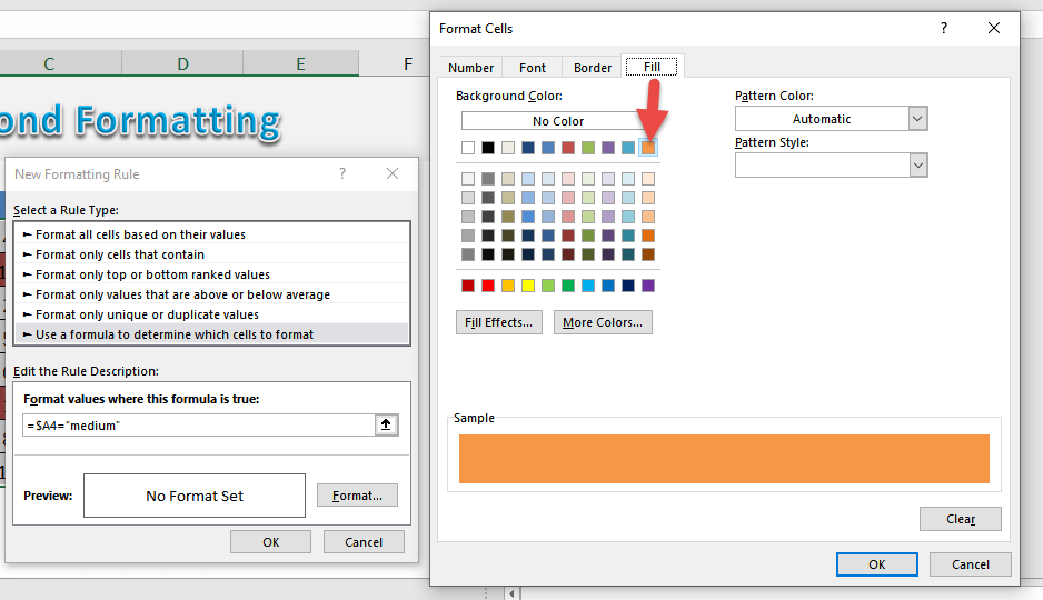
Repeat the same steps for medium values. Click New Rule.

Select Use a formula to determine which cells to format

Type in the Formula =$A4=”medium” 

This formula will ensure only the column is absolute.

Go to Format > Fill then select a color of your choosing. Click OK.

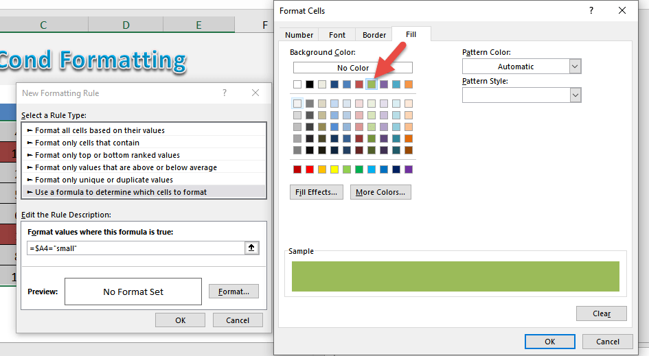
Repeat the same steps for low values. Click New Rule.

Select Use a formula to determine which cells to format

Type in the Formula =$A4=”low” 

This formula will ensure only the column is absolute.

Go to Format > Fill then select a color of your choosing. Click OK.

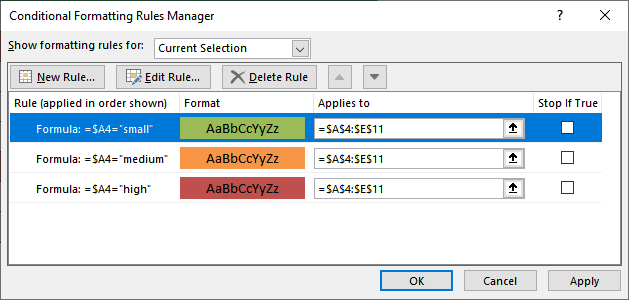
This is how our new set of rules will look like:

Now our table now has conditional formatting applied!

Advanced Tips and Tricks

Using Named Ranges for Dynamic Drop-Down Lists

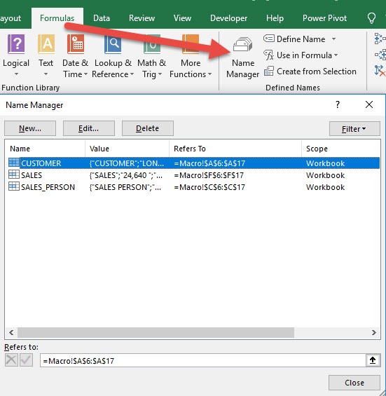
Creating dynamic drop-down lists in Excel can give your spreadsheets a polished and interactive feel. The key to this magic lies in named ranges. To begin, you’ll want to group items into a list on your sheet. Let’s say you have a list of colors on one sheet. By selecting all the colors, clicking in the Name box, and typing a one-word name like ‘ColorList’, you’re creating a named range. It’s as simple as hitting Enter.

Why do this? When you use a named range for your drop-down list, it doesn’t just make it easier to reference; it also allows your drop-down list to update automatically if you add or remove items from the range. Brilliant right?

Now, apply these named ranges to manage dynamic drop-down lists, where you can easily update and manage your data without adjusting the Data Validation settings. Just imagine, adding a new status to your project tracker or a new color to your inventory list, and it instantly becomes available in the relevant drop-down menu. This trick ensures your work in Excel is not just efficient but also error-free and adaptable to changes.

Incorporating Symbols and Icons

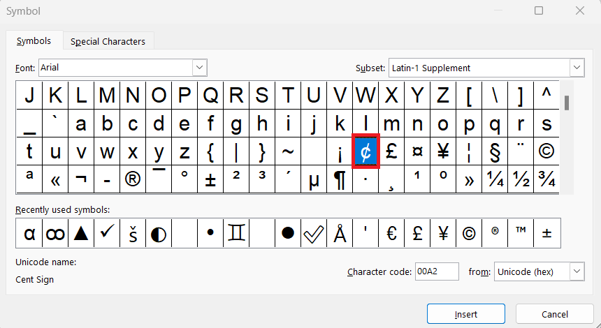
Sprucing up your Excel workbook can be quite fun when you start incorporating symbols and icons into your drop-down lists. This not only adds a visual cue but also makes the data more engaging and intuitive. Think about using a thumbs-up icon for ‘approved’ or a dollar sign for ‘budget items’. How do you do it? First, you’ll want to enable the use of Unicode characters or emojis in your workbook.

Start by finding the symbols or icons that best represent the items in your list. You can insert them directly into the cells that you’ll reference for your drop-down list. If you’re not limited by platform compatibility, emojis can work quite well here.

Once you’ve placed your symbols or icons next to the corresponding text within the cells, you simply reference these cells within your Data Validation settings. When you click on your drop-down list, you’ll delightfully see a visual representation paired with the text, making the experience of navigating through options much less mundane. You may find this particularly useful if you’re crafting forms or reports to be shared with others where clarity and engagement are paramount.

Remember to choose symbols that are easy to understand and don’t clutter your interface. A cleaner look often equates to a user-friendly experience that can dramatically enhance the navigability of your spreadsheet.

FAQ Section

Can I use different colors for each item in my Excel drop-down list?

Absolutely! Excel lets you personalize your drop-down list by applying different colors to each item. It’s a bit of a workaround using conditional formatting. Here’s how you can achieve it:

1. Define your data validation list as per usual.
2. Click on one of the cells in your drop-down list.
3. Navigate to the ‘Home’ tab and select ‘Conditional Formatting’.
4. Choose ‘New Rule’ and then ‘Use a formula to determine which cells to format’.
5. Enter the formula that corresponds to the item you’d like colored—something like =A1="YourItem".
6. Pick the formatting you desire and click ‘OK’.

You would need to repeat the conditional formatting steps for each item in the drop-down, changing the formula and colors as needed. While it takes a bit of initial setup, the result is a visually coordinated and user-friendly drop-down menu.

How to change cell color based on drop-down list?

Changing the cell color based on selections from a drop-down list is a neat trick to visually enhance your spreadsheet’s interactivity. Excel’s Conditional Formatting feature is your best friend here.

Follow these steps to start:

1. Click the cell that holds your drop-down list.
2. Go to ‘Home’, and click on ‘Conditional Formatting’, then ‘New Rule…’.
3. In the dialog box, select ‘Format only cells that contain’.
4. From the first drop-down menu, choose ‘Cell Value’ and from the second, choose ‘equal to’.
5. Type the value from the drop-down list that should trigger the color change in the next box.
6. Click the ‘Format…’ button, select the ‘Fill’ tab, and choose your color.
7. Click ‘OK’ twice to apply the rule.

Remember to create a new rule for each item and its corresponding color. This way, whenever someone selects an item from the list, the cell background changes accordingly, making your data much more digestible at a glance. It’s like having a dashboard that reacts to your inputs in real-time!

What are some best practices for using color-coded drop-down lists effectively?

To make the most out of your color-coded drop-down lists in Excel and maintain a clean, professional look, here are some best practices:

1. Consistent Color Scheme: Use a color scheme that is consistent throughout the spreadsheet to convey information clearly. Colors should have a purpose, such as red for action items or blue for informational entries.
2. Limit Color Usage: Avoid using too many colors as it can become distracting. Instead, limit the palette to a few complementary colors for readability and aesthetics.
3. Contrast for Clarity: Ensure there is enough contrast between the text color and the background color, so that the text is easily readable.
4. Color Relevance: Choose colors that logically relate to the data for intuitive understanding. For example, use green for positive values and red for negative values.
5. Accessibility Considerations: Be aware that colorblind users might interpret your color-coded lists differently. Use patterns or icons along with colors when possible.
6. Avoid Using Color Alone: To indicate status or category, use text labels or icons alongside color to ensure clarity when prints are in black and white or for those who have difficulty distinguishing colors.
7. Document the Color Code: Have a legend or a clear documentation on what each color represents, to avoid any confusion and for making your spreadsheet user-friendly.

By keeping these pointers in mind, you’ll create an Excel sheet that isn’t just functional but is also visually engaging and accessible to all users.