Rank Largest to Smallest With Excel Pivot Tables

Excel Pivot Tables have a lot of useful calculations under the SHOW VALUES AS option and one that can help you a lot is the Excel Pivot Table RANK LARGEST TO SMALLEST calculation. This option will immediately calculate the rankings (1 being the LARGEST value) for your values, allowing you to pinpoint the risks or opportunities quickly! It allows you to analyze data by ranking them and check what’s on top and what is at the bottom!

Key Takeaways

• Sort Values Quickly – Excel Pivot Tables allow you to easily sort numerical data from largest to smallest with just a few clicks, helping you spot top performers or high values instantly.

• Use the Value Field Settings – You can apply custom sorting by accessing the Value Field Settings and selecting options like “Descending” based on specific fields.

• Rank with Calculated Fields – Pivot Tables support the use of Rank formulas or DAX (in Power Pivot) to create a dynamic ranking column within the table.

• Multi-level Sorting – You can sort by one field (e.g., Sales Amount) and then apply a secondary sort on another field (e.g., Region), giving you layered sorting control.

• Dynamic Updates – Sorting from largest to smallest is automatically refreshed when underlying data changes, ensuring rankings are always up to date without manual rework.

You can easily do ranking in Pivot Table using either of the two methods mentioned below:

• Using Sorting Option
• Using Calculated Field Option

Let’s look at these methods in-depth!

Follow the step-by-step tutorial on Excel Pivot Table Rank Largest to Smallest and download this Excel workbook to practice along:

 

Using Sorting Option

STEP 1: Insert a new Pivot table by clicking on your data and going to Insert > Pivot Table > New Worksheet or Existing Worksheet

 

STEP 2: In the ROWS section put in the Sales Month field, in the COLUMNS put in the Financial Year field, and in the VALUES area you need to put in the Sales field twice, I explain why below:

 

STEP 3: Click the second Sales field’s (Sum of SALES2) drop down and choose Value Field Settings

 

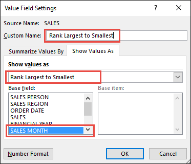
STEP 4: Select the Show Values As tab and from the drop down choose Rank Largest to Smallest.  

Select Sales Month as the Base Field. This means that we will rank the Sales Values by the Sales Month (where Rank 1 is the Largest).

Also change the Custom Name into Rank Largest to Smallest to make it more presentable.  Click OK.

 

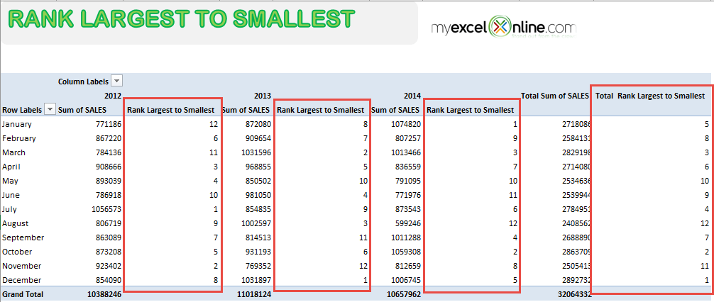
You now have your Pivot Table, showing the Rank Largest to Smallest for the sales data of years 2012, 2013, and 2014.

You can see that each red box is the ranking for each year (for Years 2012, 2013, 2014, and the Total Rankings).

This is how you can easily Rank Pivot Table in few easy steps!

 

Using Calculated Field

STEP 1: Select any cell in the data and then Go to Insert > Pivot Table.

STEP 2: In the dialog box, select New Worksheet and then click OK.

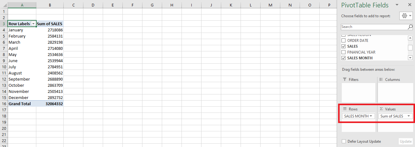
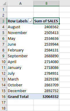
STEP 3: Drag and drop Sales Month in the Row field and Sales in the Values field.

STEP 4: Click on the filter button and Select More Sorting Option.

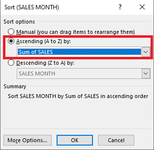
STEP 5: In the Sort dialog box, Select Sum of Sales in the Ascending by dropdown. Click OK.

This will sort the data in ascending order!

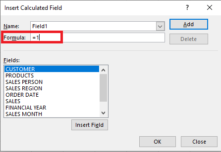
STEP 6: Click on any cell in the Pivot Table and Go to PivotTable Analyze > Calculated Field.

STEP 7: In the Insert Calculated Field dialog box, Type =1 n the formula field. Click OK.

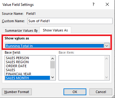
STEP 8: Right-Click on the calculated field and select Value Field Setting.

STEP 9: In the Value Field Setting dialog box, Select Running Total in as Show Value as! Click OK.

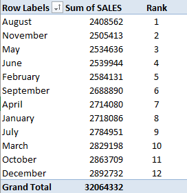
This will sort the values from largest to smallest and insert a rank field in the Pivot Table!

Frequently Asked Questions

How do I sort data from largest to smallest in a Pivot Table?
Right-click on any numeric value in the Pivot Table, choose Sort → Sort Largest to Smallest, and Excel will automatically reorder the rows accordingly.

Can I rank items within each category in a Pivot Table?
Yes, you can enable multi-level sorting by dragging category fields into Rows and then sorting values within each category individually.

Is it possible to show the rank number directly in a Pivot Table?
Yes, by using Rank formulas or DAX functions in Power Pivot, you can display a ranking number alongside each item based on your sorting criteria.

Will the sorting update if I change the source data?
Absolutely. When you refresh the Pivot Table, the largest-to-smallest sort order automatically updates to reflect any new or changed data.

Can I sort text fields alphabetically after sorting numbers?
Yes, Excel allows you to sort numerical fields by size and then sort text fields alphabetically, giving you flexible control over how your Pivot Table is organized.

Conclusion

In this tutorial, you have learned how to rank in pivot table by either using the Sorting option or by inserting a calculated field.