Exercise Workbook:
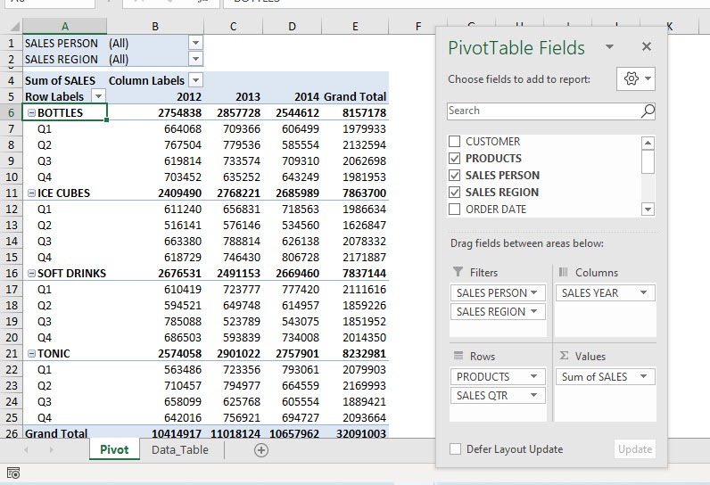
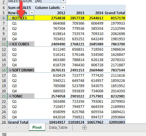
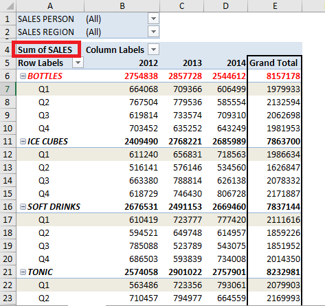
Here is our current Pivot Table:
Enable Selection in Pivot Table
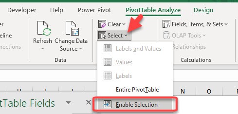
STEP 1: To enable this, go to PivotTable Analyze > Actions > Select > Enable Selection
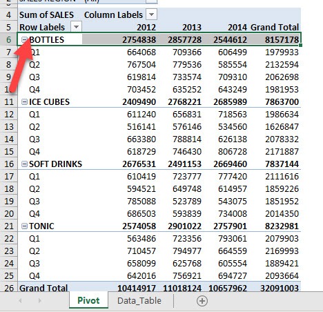
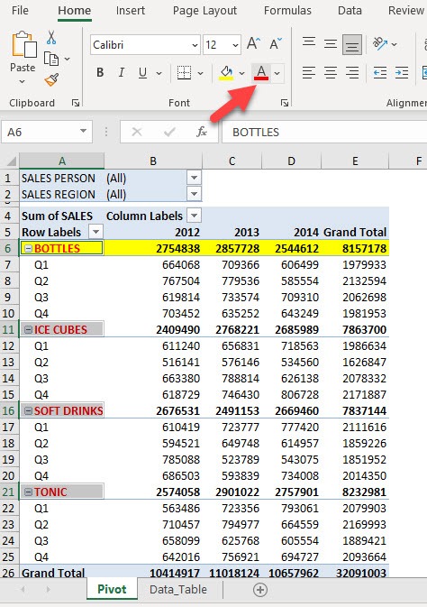
STEP 2: Let us try it out! Select the Bottles Product from the left-hand side to highlight it.
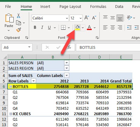
Make any formatting change and it will apply to the entire Bottles Product. So this means we have targeted a specific product.
STEP 3: What if we want to apply a formatting change to all Product Labels in one click? Click on the top portion of Bottles.
You will see all of the Product Labels got highlighted. Make any formatting change.
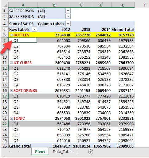
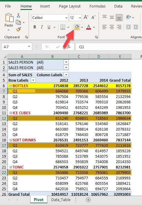
STEP 4: Let us now try on a specific quarter. Select the left-hand side of Q1 to select it.
Make any formatting change. And all Q1 values will immediately have this formatting change.
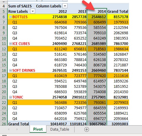
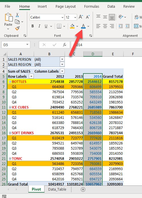
STEP 5: You can do the same for a specific column. Click the 2014 column.
Make the formatting change, and see the effects happen instantaneously!
Once you have enabled selection in Pivot Table, you can easily apply formatting to any section.
You can also use selection arrows to select the entire Pivot Table by following the steps below:
STEP 1: Move the cursor to the top-left cell of the Pivot Table
STEP 2: Once the cursor changes to an arrow, click on the cell.
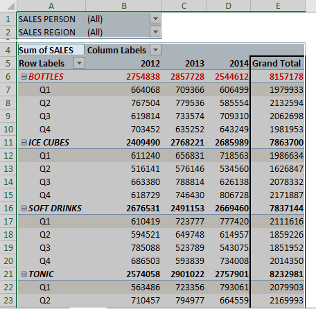
The entire Pivot Table will be selected.
Want an easier way than this? Luckily, Excel has that too!
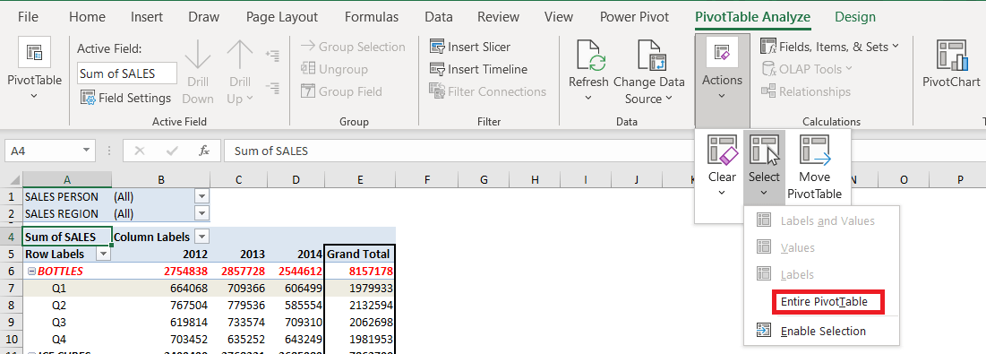
Go to PivotTable Analyze > Actions > Select > Entire PivotTable
The entire Pivot Table will be selected.
Click here to know Top 50 things that you can do with Excel Pivot Table!
Make sure to download our FREE PDF on the 101 Best Excel Tips & Tricks:

Bryan
Bryan Hong is an IT Software Developer for more than 10 years and has the following certifications: Microsoft Certified Professional Developer (MCPD): Web Developer, Microsoft Certified Technology Specialist (MCTS): Windows Applications, Microsoft Certified Systems Engineer (MCSE) and Microsoft Certified Systems Administrator (MCSA).
He is also an Amazon #1 bestselling author of 4 Microsoft Excel books and a teacher of Microsoft Excel & Office at the MyExecelOnline Academy Online Course.
