Show The Percent of Parent Column Total With Excel Pivot Tables

Excel Pivot Tables have a lot of useful calculations under the SHOW VALUES AS option and one that can help you a lot is the PERCENT OF PARENT COLUMN TOTAL calculation. This option will immediately calculate the percentages for you from a table filled with numbers such as sales data, expenses, attendance, or anything that can be quantified.

 

Why Use Percent of Parent Column Total?

Let’s face it—big tables full of numbers can be overwhelming. What you really want is insight. This calculation transforms raw values into meaningful percentages that show contribution within hierarchical categories. Imagine you’re tracking sales across multiple years, broken down by quarter and salesperson. Sure, you could see that John sold $50,000 in Q2 of 2013, but that number alone doesn’t tell you how big his share of Q2 2013 sales was. Was it 5%? 25%? 50%?

With Percent of Parent Column Total, you can immediately see John’s contribution relative to the quarter’s subtotal, without writing a single formula.

How to Show The Percent of Parent Column Total With Excel Pivot Tables

STEP 1: Insert a new Pivot table by clicking on your data and going to Insert > Pivot Table > New Worksheet or Existing Worksheet

 

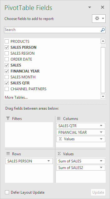
STEP 2: In the ROWS section put in the Sales Person field, in the COLUMNS put in the Sales Qtr and Financial Year fields and in the VALUES area you need to put in the Sales field twice, I explain why below:

 

STEP 3: Click the second Sales field’s (Sum of SALES2) drop down and choose Value Field Settings

 

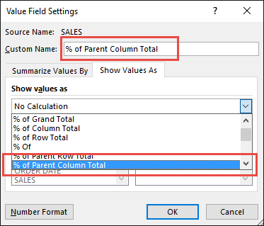
STEP 4: Select the Show Values As tab and from the drop down choose % of Parent Column Total. 

Also change the Custom Name into % of Parent Column Total to make it more presentable. Click OK.

 

STEP 5: Notice that the % of Parent Column Total data is in a decimal format that is hard to read:

 

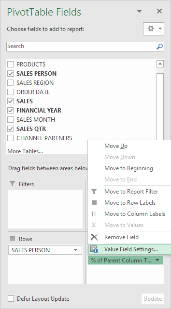
To format the % of Parent Column Total column, click the second Sales field’s (% of Parent Column Total) drop down and choose Value Field Settings. 

The goal here is for us to transform numbers from a decimal format (i.e. 0.23), into a percentage format that is more readable (i.e. 23%).

 

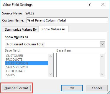
STEP 6: Click the Number Format button:

 

 

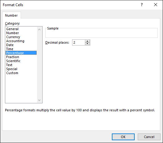
STEP 7: Inside the Format Cells dialogue box, make your formatting changes within here and press OK twice.  

In this example, we used the Percentage category to make our % of Parent Column Total numbers become more readable.

 

You now have your Pivot Table, showing the % of Parent Column Total for the Sales data of years 2012, 2013, and 2014 grouped by Quarters.

All of the Sales numbers are now represented as a Percentage of its Parent’s Subtotal i.e. Percentage of each Quarter’s Subtotal.

You can see that the red boxes are represented as 100% in totality when grouped together for each Quarter (encapsulating blue box):

Click on the image to enlarge…

 

Benefits of Using This Feature

• Saves Time – No need to create complex formulas with SUMIFs or nested logic.
• Dynamic Updates – If you add new data and refresh, the percentages recalculate instantly.
• Better Presentations – When sharing with managers, percentages are easier to digest than raw figures.
• Supports Comparisons – Quickly see who’s contributing more or less over different quarters or years.
• Works Across Data Types – Whether it’s revenue, headcount, inventory, or costs, it adapts to your dataset.

 

Common Mistakes to Avoid

• Using it on single-level data – This feature shines when there are parent-child relationships (e.g., Category > Subcategory). If you only have one column field, you won’t see meaningful results.
• Confusing it with % of Column Total – These are not the same. “% of Column Total” looks at the whole column, while “% of Parent Column Total” limits the calculation to the immediate parent group.
• Forgetting to format as a Percentage – Leaving decimals like 0.25 instead of 25% makes your Pivot Table less readable.
• Not renaming fields – Always rename the second field to “% of Parent Column Total” so your Pivot Table doesn’t look cluttered.

 

Frequently Asked Questions

Where do I find the ‘Percent of Parent Column Total’ option in Excel Pivot Tables?

The % of Parent Column Total option is located under the Show Values As menu within Pivot Tables. To access it:

• Right-click on any numeric value inside your Pivot Table.
• From the context menu, choose Show Values As.
• You’ll see a list of calculation options—select % of Parent Column Total.

This will transform the selected field into percentages that reflect each item’s contribution to its immediate parent group, instead of showing the raw numbers. For instance, if you have “Quarter” and “Year” in your column fields, each Quarter’s percentages will be calculated relative to its parent Year.

Can I use this option if I only have one column field?

No. The Percent of Parent Column Total calculation is specifically designed for hierarchical data—meaning data that has multiple levels of grouping in the column area. If you only have one column field, Excel doesn’t have a “parent” category to compare against, so the calculation won’t work as expected.

What’s the difference between ‘% of Column Total’ and ‘% of Parent Column Total’?

• % of Column Total = compares each value against the entire column total.
• % of Parent Column Total = compares each value against its immediate parent group only.

Think of it as: Column Total = big picture, Parent Column Total = local context.

Will this percentage update if I filter the Pivot Table?

Yes, absolutely. One of the strengths of Pivot Tables is that calculations like % of Parent Column Total are dynamic. If you apply filters—whether slicers, report filters, or manual selections—Excel automatically recalculates percentages based on the visible data only.

Can I apply this to multiple fields at once?

Yes, you can. The % of Parent Column Total calculation is not limited to a single field. If you want to show it for multiple metrics (e.g., Sales, Profit, Expenses), you can do so by repeating the following steps for each field:

• Drag the metric into the Values area.
• Right-click the field, choose Show Values As, and select % of Parent Column Total.
• Rename the field for clarity (e.g., “% of Parent Sales,” “% of Parent Profit”).

This way, you can present both raw numbers and relative percentages side by side, giving your audience a more complete picture of the data.