Show The Difference From Previous Months With Excel Pivot Tables

STEP 2: Insert a new Pivot table by clicking on your data and going to Insert > Pivot Table.

STEP 4: In the ROWS section put in the Sales Month field, in the COLUMNS put in the Financial Year field and in the VALUES area you need to put in the Sales field twice, I explain why below:

The Pivot Table will look like this:

Visual Aids: Enhancing Your Month-to-Month Data

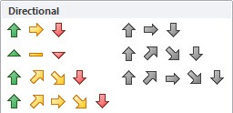
Directional Icons for Quick Insights

Visual aids play a crucial role in the comprehension of data, more so when you want to depict changes over time, like month-to-month fluctuations. By incorporating directional icons into your pivot tables, you equip your audience with the ability to capture the essence of the data at a glance. Imagine icons that rise or dip, offering immediate insight into trends without poring over each number—this is the convenience directional icons offer. They represent increases, decreases, and steadiness with upward arrows, downward arrows, and dashes, respectively.

Conditional Formatting for Clarity and Impact

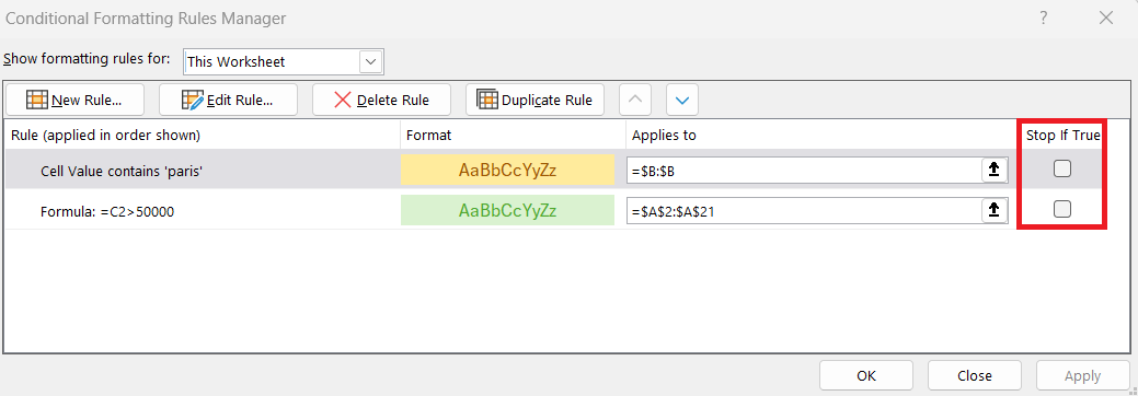
Conditional formatting can dramatically increase the clarity and impact of your data visualization. With Excel’s rich set of formatting rules, you can highlight month-to-month changes in a way that brings immediate attention to important trends. For example, you might use a gradient color scale to show varying degrees of increase or decrease, or apply a specific color to represent significant shifts. To set this up, simply select the % change column in your pivot table, navigate to “Home > Conditional Formatting > New Rule,” and specify your rule to reflect the desired visual effect.

Advanced Tips for Pivot Table Magic

Dealing with Common Errors and Issues

Working with pivot tables to show month-to-month changes often leads to encounters with errors or unexpected results, especially when using ‘Difference From’ or ‘% Difference From’ settings. Errors might manifest as baffling messages, or you could observe issues when attempting changes. To navigate around these bumps, an understanding of why these errors arise is invaluable.

A common error may be a result of data fields moving or becoming renamed, leading to invalid references. Always double-check your data sources and field names. Another hiccup occurs when calculations on blank cells or zeroes return errors or divide-by-zero results. In this case, ensure you have complete data or consider using custom formulas that account for these possibilities.

Leveraging More Pivot Table Value Settings

Diving deeper into pivot table value settings opens up a universe of data analysis possibilities. You’re not just limited to displaying sums or counts; you can customize your pivot table to perform a variety of calculations, such as averages, maximums, minimums, or more sophisticated computations like running totals or percentiles.

To access these, right-click on a value within your pivot table and explore the ‘Summarize Values By’ and ‘Show Values As’ options. For month-to-month analysis, you might select ‘Difference From’ to view the absolute change or ‘% Difference From’ for the relative change from one month to the next. Each selection dynamically reshapes your data’s story, giving you the analytical edge.

FAQ: Excel Pivot Magic – Your Questions Answered

How do I set up my pivot table to show month-to-month changes?

To set up a pivot table that shows month-to-month changes, you need to group your date data by months and years first. Right-click on a date within your PivotTable, choose ‘Group’, then select both ‘Months’ and ‘Years’. Add your data field, say ‘Sales’, to the ‘Values’ area twice. Name one as ‘Total Sales’ and the other as ‘% Change’. Set the second field to show ‘values as’ “% Difference From”, choosing ‘Month’ as the Base field and ‘(previous)’ as the Base item. This will calculate the percentage change from one month to the next.

What are some common errors when using ‘Difference From’ in pivot tables, and how can they be fixed?

Common errors when using ‘Difference From’ in Excel PivotTables often stem from empty cells, incorrect fields, or data changes. If you run into an error, first check your data source to ensure it’s complete without blanks in crucial areas. Also, verify that the Base Field and Base Item are correctly set and still present in the PivotTable—adjustments or removals can lead to errors. If you encounter #DIV/0! errors, it usually means you’re trying to calculate a difference with a zero value. In such cases, you might need to review your data preprocessing steps or include safeguards in your calculations to manage zeroes appropriately.

Can I use pivot tables to show percentage differences as well?

Absolutely, pivot tables are equipped with functionality to show percentage differences, which can provide you with deep insights into your data’s trends over time. To do this, add a field to your pivot table’s values area twice. Right-click on the second instance of this field, select ‘Show Values As’, and then choose ‘% Difference From’. You’ll need to pick a base field, like the month or year, depending on your data, and then Excel will compute the percentage change for you relative to the base field you’ve selected.