Show Report Filter Pages in a Pivot Table

When you are using an Excel Pivot Table, you can create separate reports for each department, region, or category. Excel has a useful feature called Show Report Filter that can automatically create separate reports. In this article, you will learn how to use Show Report Filter Pages in a Pivot Table.

Key Takeaways:

• Show Report Filter Pages creates separate worksheets automatically.
• Each filter item gets its own Pivot Table report.
• You need to add a field to the Filters area first.
• All Pivot Tables remain connected to the same source data.
• Use Refresh All to update the Pivot Table reports.

 

What is Show Report Filter Pages in Excel?

The Show Report Filter Pages feature creates a new worksheet for each item available in a Pivot Table report filter. Excel automatically copies the Pivot Table layout and applies a different filter item to each worksheet. This allows you to quickly view individual reports without changing the filter again and again.

For example, suppose I have sales data for four regions:

• East
• West
• North
• South

If you add Region as a filter in the Pivot Table, you can use Show Report Filter Pages to create four separate worksheets. Each worksheet will display the sales data for one region only. The worksheet names are also based on the filter items, making the reports easy to identify

 

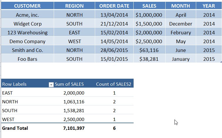
Our Pivot Table Setup

How to Show Report Filter Pages in a Pivot Table

STEP 1: Drop the Customer Field in the report filter.

 

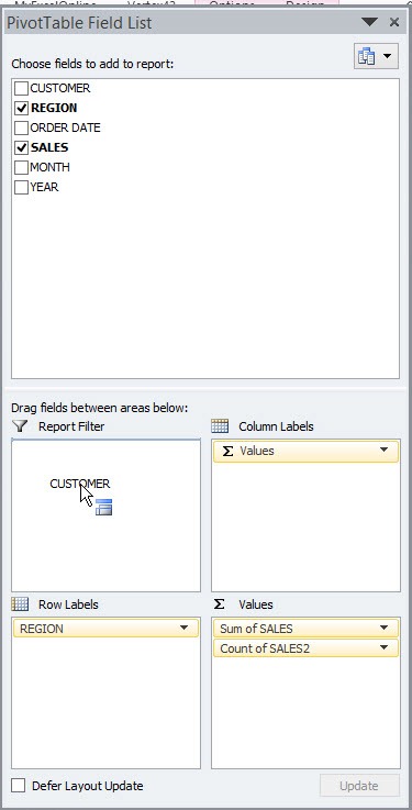
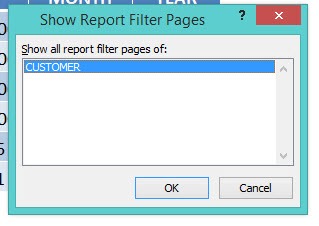
STEP 2: Go to Options > Options Drop Down > Show Report Filter Pages

 

STEP 3: Press  OK.

Each customer’s pivot table will show in a unique sheet!

 

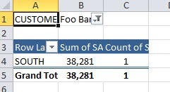
Refresh Pivot Tables After Source Data Changes

If the source data changes, the Pivot Tables also need to be updated. To refresh the Pivot Table,

• Click anywhere inside a Pivot Table.
• Go to the Data tab.
• Click on Refresh All.

This updates the Pivot Table results using the latest source data.

Tips & Tricks

• Show Report Filter Pages only works with fields placed in the Filters area of the Pivot Table.
• The feature creates a separate worksheet for every filter item.
• All worksheets use the same Pivot Table layout.
• New worksheets are added to the current workbook.
• If new filter items are added later, you may need to run the feature again.
• You should check the number of unique filter items before using the feature.

 

Frequently Asked Questions

What is the “Show Report Filter Pages” feature in Excel Pivot Tables?

The Show Report Filter is a tool that automatically creates a separate worksheet for each item in the report filter. It uses the same Pivot Table structure for each sheet.

Where to find the “Show Report Filter Pages” option?

To find Show Report Filter Pages,

• Go to the PivotTable Analyze tab
• Click on Options
• Click Show Report Filter Pages
• Select the filter field you want to split by.

Can I use multiple filter fields with Show Report Filter Pages?

No, it works with only one filter field at a time. However, you can repeat the process for different fields if needed.

Are the generated sheets linked to the source data?

When you create multiple Pivot Tables using the Show Report Filter pages option, all the Pivot Tables are connected to the same data source.

What happens if I add new items to the filter field later?

New filter items won’t automatically generate new sheets. You will have to run Show Report Filter Pages again to create reports for the newly added items. Excel will then create report pages for the new filter items based on the updated Pivot Table data.