The Ultimate Guide to Sum Formula and AutoSum Feature in Excel

Excel is more than just a tool for basic arithmetic; it’s a robust platform for analyzing and computing complex data sets. With Microsoft Excel, you can perform intricate calculations, identify trends, and even forecast future values—all within a single spreadsheet. At the heart of these capabilities are sum formulas and the AutoSum feature, which simplify the process of adding up numbers, making Excel an essential tool for data management and analysis.

Key Takeaways:

• Efficient Data Summation: Excel’s SUM function and AutoSum feature allow for quick and accurate summation of data ranges, reducing the risk of manual errors.
• Handling Complex Criteria: Functions like SUMIF and SUMIFS enable summing based on specific conditions, providing powerful tools for targeted data analysis.
• Managing Non-Contiguous Cells: Excel can sum non-adjacent cells easily, offering flexibility in how data is processed and displayed.
• Error Management: With functions like IFERROR, Excel ensures smooth summation even when dealing with cells that contain errors.
• Advanced Summation: The SUMPRODUCT function and other advanced formulas extend Excel’s summing capabilities to more complex data analysis scenarios, allowing for multi-criteria calculations and array operations.

 

Introduction to Excel Summation Tools

Essentials of Excel’s Calculating Capabilities

Excel goes far beyond the basic math you might do on a calculator; it’s a powerful tool for analyzing and computing complex data sets. You can perform calculations on numbers, pinpoint trends, and even forecast future values all within your spreadsheets.

Overview of Sum Formulas and AutoSum Feature

Sum formulas are integral to Excel, giving you the ability to quickly add up numbers within your spreadsheet. Whether you’re dealing with sales figures, inventory counts, or financial data, these formulas work seamlessly to provide instant totals.

The AutoSum feature takes this convenience further by automating the summing process. With a single click (or a swift keyboard shortcut), Excel identifies the range of cells you’re working with and applies the SUM function for you, streamlining your workflow and reducing the risk of manual errors.

 

Exploring Excel’s SUM Function

The Basics of Using the SUM Function

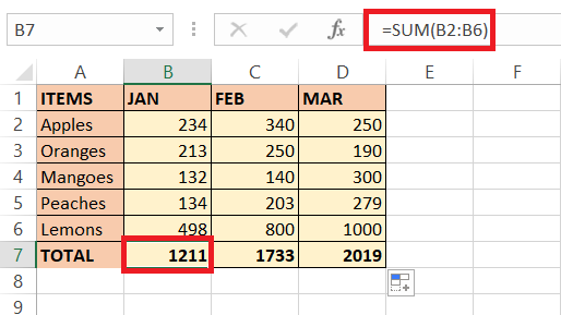
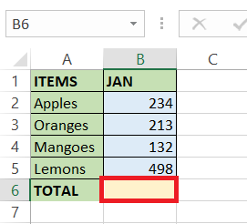
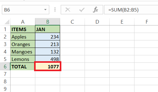
Getting a grip on the SUM function in Excel is like having a Swiss Army knife for your data—it’s versatile and essential. To start summing up numbers, you’ll usually select a range of cells you want to tally. It’s as simple as typing =SUM, followed by your chosen cells embraced in parentheses. For example, =SUM(B1:B6) swiftly provides the total of cells from B1 to B6.

NOTE: Remember, you can also click and drag to select a range instead of typing it out. Excel is smart enough to figure out what you’re trying to do and helps by completing the formula.

Syntax and Examples for SUM

When you’re ready to dive into the nuts and bolts, understanding the syntax is crucial. The setup goes like =SUM(number1, [number2], ...), where number1 is mandatory, and subsequent numbers (up to 255 additional arguments) are optional. You can feed this function cell references or actual numbers.

Let’s see some examples in action:

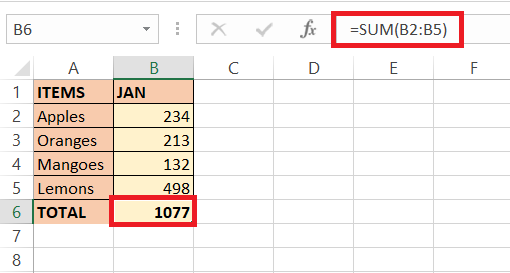
• =SUM(B2:B5) quickly totals the first four cells in the A column.

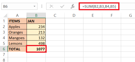
• =SUM(B2, B3, B4, B5) sums up the first cell from columns A, B, and C.

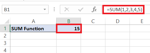
• =SUM(1, 2, 3, 4, 5) simply adds up these five numbers, giving you 15.

Flexible enough to sum continuous ranges or individual cells, the SUM function adapts to your needs, making it a fundamental feature for robust data management.

 

The Power of AutoSum Magic

How AutoSum Simplifies Adding in Excel

AutoSum is like your quick-add assistant; it’s the fastest way to sum up a column or row of numbers. Once clicked, it automatically enters a SUM function for the selected cells. What’s neat is that Excel anticipates your range, often correctly guessing the cells you aim to total. If it’s ever off-track, you can easily adjust the selection and press Enter to confirm.

This feature isn’t just about speed; it also helps reduce the potential for slip-ups that can happen when entering formulas manually, making sure your totals are accurate without the fuss.

Steps to Utilize AutoSum Effectively

To harness the power of AutoSum, follow these steps and watch your data summarizing go from painstaking to pain-free:

STEP 1: Click the cell where you want the sum to appear. This is typically right below a column of numbers or to the right of a row.

STEP 2: Hit the ‘AutoSum’ button (usually found in the ‘Home’ tab within the ‘Editing’ group) or press ALT + = if you appreciate keyboard shortcuts.

STEP 3: Excel will automatically select the most likely range of cells it thinks you want to total. If it’s not quite right, you can adjust the range by clicking and dragging as needed. If you’re adding rows and columns, you might be pleased to see Excel insert multiple SUM functions across the range.

RESULT: Use AutoSum to rapidly generate totals, whether it’s your monthly sales or a comprehensive financial report—Excel has your back.

 

Advancing with AutoSum: Tips and Tricks

Summing Non-contiguous Cells with Ease

If the cells you need to add aren’t side by side, fret not! Excel has got you covered. Summing non-contiguous (separate) cells is just as simple as handling a continuous range. Just use the SUM function and separate each cell reference with a comma.

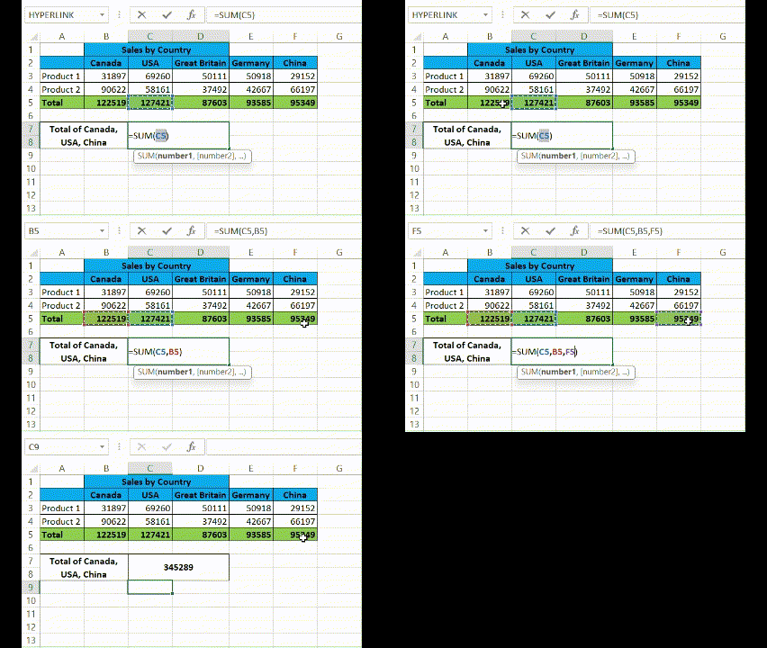
For instance, =SUM(B5, C5, F5) quickly tallies the numbers in cells B2, C5, and F8. And here’s a little secret: it works exactly like summing a range—=B5+C5+F5 is your alternative shortcut.

Let’s look at the steps below to undertake the same:

STEP 1: Select the cell where you want your result. Then click on “AutoSum”.

STEP 2: Hold down CTRL key and start selecting the cells needed for your calculation, here Sales of Canada, USA & China. Then press ENTER to complete the formula.

Beyond Basic Summing: Advanced Formulas

Tackling Complex Criteria with SUMIF and SUMIFS

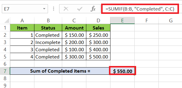
When your data set starts getting a bit more picky, and you need to sum cells that meet specific criteria, the SUMIF and SUMIFS functions swing into action like financial superheroes. SUMIF is great for a single condition. You’ll give it a range, a criterion, and an optional sum range, such as =SUMIF(B:B, "Completed", C:C) to add up all values in column C where column B reads “Completed.”

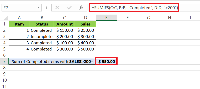
Escalate the game with SUMIFS when you’ve got multiple conditions to meet. This function orders the criteria right after your sum range, like, =SUMIFS(C:C, B:B, "Completed", D:D, ">200"), which adds up all the values in column C where column B is “Completed” and column D is greater than 200.

Get ready to embrace the orderliness and power of focused summing with these two trusty functions by your side.

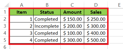
Example Dataset:-

Perform the below steps to understand deeper into this;

• To sum all “Completed” items’ amounts, use “=SUMIF(B:B, “Completed”, C:C)”.

• To sum amounts where Status is “Completed” and Sales are over 200, employ “=SUMIFS(C:C, B:B, “Completed”, D:D, “>200″)”. You’ll get the sum of $550 (150+100+300).

SUMPRODUCT: Adding with Conditions on Steroids

Think of SUMPRODUCT as the Swiss Army knife on steroids when it comes to conditional adding in Excel. Summing with conditions? Check. Counting with multiple criteria? Check. Even array operations? Check again!

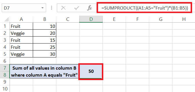
Unleash its capability with a formula that might look a tad complex, but is powerful: =SUMPRODUCT((A1:A10="Fruit")*(B1:B10)), adds up all the values in B1:B10 where A1:A10 cells equal “Fruit”. It’s the go-to tool for when your data analysis demands that extra oomph.

Example Dataset:-

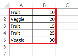
• To sum all values in column B where column A equals “Fruit,” use “=SUMPRODUCT((A1:A5=”Fruit”)*(B1:B5))”. The formula will return 50, as it sums 10, 15, and 25, the values corresponding to “Fruit” in column A.

Bear in mind though, SUMPRODUCT doesn’t take kindly to pesky text or error values within the arrays, so keep your data clean for this function to showcase its full potential.

 

Handling Exceptional Case in Summation: Adding Cells with Errors or Specific Formats

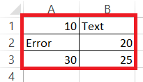
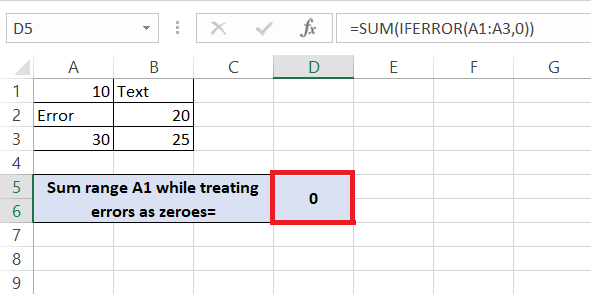
If you’ve faced the frustration of error values throwing a wrench in your summing plans, fret not—Excel offers elegant solutions. For the brave souls working with ranges that may contain errors, wrap your numbers in the IFERROR function along with your SUM, like so: =SUM(IFERROR(A1:A10,0)). This formula conveniently treats any errors as zeroes, ensuring a smooth summing process.

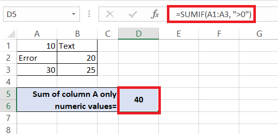
Example Dataset:-

• To sum the range A1, while treating errors as zeroes, use “=SUM(IFERROR(A1:A3,0))”.

• To sum only cells with numeric values in column A, apply Conditional Formatting to highlight them. Then, use “=SUMIF(A1:A3, “>0″)” to sum only the cells with numeric values.

 

FAQs: Mastering Sum Formulas & AutoSum in Excel

How to Quickly Access the AutoSum Feature?

To quickly access the AutoSum feature, click the cell where you’d like your total, then head to the ‘Home’ tab and click on the ‘AutoSum’ button. Alternatively, skip the navigation and simply press ALT + = on your keyboard for instant access. Whichever route you choose, AutoSum is a click or shortcut away, ready to tally up your numbers in a flash.

What Is the Difference Between SUM and SUMIF functions?

SUM adds up all the numbers in a specified range, while SUMIF sums only the ones that meet a criteria you define. Use SUM when you want a straightforward total, and reach for SUMIF when you’re only interested in adding numbers that pass a certain test, like sales greater than $100.

Can AutoSum Handle Text and Error Values?

Yes, AutoSum skillfully ignores any text in the selected range. However, when encountering cells with errors, it will not be able to provide a sum and will return an error instead. If you come across this, consider using the AGGREGATE function, which can sum while ignoring errors, to keep your productivity on track.

How to write a sum formula in Excel?

To write a sum formula, start by typing an equals sign (=) into the cell where you want the total, followed by the word SUM. Then, open a parenthesis, select the range of cells you want to add, close the parenthesis, and press Enter. For example, =SUM(A1:A10) adds up values from cell A1 to A10.

How do I calculate the total sum in Excel?

To calculate the total sum in Excel, you can either use the SUM function or the AutoSum feature. Click the cell where you’d like to see the total, then click the AutoSum button in the ‘Home’ tab or type =SUM(range) where ‘range’ is the group of cells you’re adding up. Hit Enter, and the total is calculated.