Avoid Errors: Learn Excel IFERROR Function with Easy Examples

Mastering the IFERROR function in Microsoft Excel is a game-changer for creating professional and error-free spreadsheets. This guide will equip you with a thorough understanding of how to implement IFERROR to manage errors seamlessly, enhancing the reliability of your data analysis. Follow these steps to skillfully navigate common Excel errors and present your data with confidence.

Key Takeaways

• The Excel IFERROR function is essential for managing errors, especially in complex worksheets, by providing an option to display alternative text instead of error messages.
• Utilizing IFERROR helps in creating spreadsheets that are visually clean and understandable, which is particularly advantageous when presenting data to others.
• IFERROR simplifies the troubleshooting process by identifying problematic formulas and allowing for the insertion of custom error messages.
• Learning to use the IFERROR function can significantly enhance Excel proficiency and contribute to the production of more dependable spreadsheets.

Download the workbook and follow along with the tutorial on IFERROR Function in Excel – Download excel workbookMaster-Excel-IFERROR-Function-with-Easy-Examples.xlsx

 

Introduction to Excel’s Error Handling

What Is the IFERROR Function?

The IFERROR function in Microsoft Excel is a powerful tool for managing errors within spreadsheet calculations. It streamlines the process of error checking by combining error detection and alternative actions into a single, unobtrusive function.

In essence, the IFERROR function evaluates a specified expression and determines whether it results in one of several common error types such as #N/A, #VALUE!, #REF!, #DIV/0!, #NUM!, #NAME?, or #NULL!. If an error is found, instead of displaying the standard error message, IFERROR enables Excel to return a value or perform an action that you designate.

The genius of IFERROR lies in its simplicity and effectiveness in preventing error messages from disrupting the appearance and functionality of your spreadsheets. It allows users to maintain a clean dataset and ensures that subsequent formulas dependent on the initial results are not derailed by unexpected errors.

By employing the IFERROR function, Excel users can make their formulas more robust and their outputs more presentable, offering both aesthetic and practical advantages when working with complex data.

 

Syntax and Parameters for Using IFERROR

Understanding how to properly use the IFERROR function requires familiarity with its syntax and parameters. Here’s how the function is structured:

Where the parameters are defined as follows:

• value: This argument represents the formula or expression you wish to test for errors. It can be any formula that might produce an error from which you want to protect your worksheet.
• value_if_error: This is the value or action that the IFERROR function will return or execute if it detects an error in the value argument. This could be a custom message like “Error found,” a numerical substitute such as 0, a blank cell indicated by "", or even another formula.

The IFERROR function works by first attempting to execute the formula specified in the value parameter. If this computation is error-free, the formula’s result is returned just as it would be without the IFERROR function. However, if an error is encountered during the computation, the value_if_error parameter comes into play, and its contents are returned by the function instead.

The robustness of the IFERROR function allows for a broad range of scenarios where error handling is crucial, paving the way for more reliable data management and presentation.

 

Practical Application: IFERROR in Action

Example 1 – Avoiding the #DIV/0! Error in Division Calculations

When working with Excel spreadsheets, division calculations are common, and a frequent error encountered during these operations is the #DIV/0! error. This error occurs when a formula tries to divide a number by zero or a blank cell, a mathematically undefined operation.

Here’s a practical scenario: you have a spreadsheet that calculates the unit price of items by dividing the total cost by the quantity. If the quantity is zero or a cell is left blank, Excel will return a #DIV/0! error. This can be distracting and create confusion when analyzing the resultant data.

Using the IFERROR Function to Avoid the #DIV/0! Error:

In this example, A2 represents the plumbing complaints, and B2 is the cell containing the plumbers on duty. The formula is divided into two parts:

• The division operation A2/B2 is what you’re trying to calculate.
• The "Not Available" text (which could also be a 0 or an empty string "") is what Excel will output if the result of the division is a #DIV/0! error.

If B2 contains a number other than zero, Excel will successfully perform the division and return the unit price. However, if B2 is zero or blank, the IFERROR function will intervene and return “Not Applicable” instead of the default error message.

This effectively handles the error by providing a readable and sensible placeholder, ensuring continuity of your data analysis and averting confusion that could arise from seeing raw error codes in your worksheet.

Example 2 – Handling VLOOKUP Errors Gracefully

VLOOKUP is one of Excel’s most widely used functions, particularly for finding specific values in a dataset. However, it is just as notorious for generating #N/A errors when a lookup value is not found. Fortunately, the IFERROR function can be utilized to handle these VLOOKUP errors gracefully.

Consider a data set of student names with accompanying marks. We’ll use the VLOOKUP function to find the marks for specific students. But if we try to look up a name that doesn’t exist in the dataset, Excel will return the #N/A error. This is when the IFERROR function comes into play.

Using IFERROR with VLOOKUP to Manage Errors:

In this example:

• E2 contains the student’s ID we’re searching for.
• $A$2:$C$6 is the range where the first column ($A$2:$A$6) contains the student ID, and the second column ($B$2:$B$6) contains the GPA and third column ($C$2:$C$6).
• 3 indicates that we want to retrieve the value from the second column of the range.
• FALSE specifies that we want an exact match for the lookup.
• "Not Found" is the text that will replace the #N/A error if VLOOKUP fails to find the student’s name within the specified range.

 

When a matching name is found, VLOOKUP functions normally and returns the corresponding mark. If the lookup fails, IFERROR catches the #N/A error and ensures that “Not Found” is displayed rather than the default error code. This provides clarity and prevents dataset users from encountering uninformative error messages.

The syncing of IFERROR with VLOOKUP enhances the robustness of data retrieval processes, helping maintain a refined and user-friendly Excel environment.

 

Advanced Tips for IFERROR Users

Nested IFERROR: Layered Error Checking

Nested IFERROR functions in Excel allow for layered error checking, offering a multi-tiered approach to error handling. This technique is particularly useful when you have formulas that could generate different types of errors, or when a simple pass/fail response isn’t sufficient and you need a sequence of fallbacks. By nesting IFERROR functions, you create a cascade of error checks, where each layer addresses a potential error in turn.

Example of Nested IFERROR Functions:

Let’s consider a scenario where you’re using a combination of functions like VLOOKUP and INDEX/MATCH that may produce different errors. You want to first try VLOOKUP, then INDEX/MATCH, and if both fail, you want to return a message like “Not found”.

=IFERROR(VLOOKUP(E1,$A$2:$C$7,3,FALSE),IFERROR(INDEX(A2:C7,MATCH(E1,C2:C7,0),2),”Not Found”))

In this nested structure:

• The first VLOOKUP attempts to find lookup_value in table_array1 and return the value from the specified column col_index_num.
• If VLOOKUP fails and results in an error, the first IFERROR catches it and then proceeds to the nested IFERROR.
• Within the nested IFERROR, the INDEX/MATCH combo executes, offering a second chance to retrieve the data.
• If both functions lead to an error, the second IFERROR comes into play, ultimately outputting “Not found” instead of an error code.

This approach allows each step to act as a safety net for the previous one, ensuring that all reasonable methods to retrieve the data are exhausted before delivering a custom message. Using nested IFERROR functions adds depth to error handling in Excel, allowing for more sophisticated and resilient formula creation.

 

Alternative Functions: IFERROR vs. ISERROR

Comparing IFERROR with ISERROR is essential for Excel users seeking a comprehensive approach to managing errors in their spreadsheets. While both functions are designed for error detection, they function quite differently and serve unique purposes.

ISERROR Function Overview:

The ISERROR function is employed purely for the identification of errors. It checks whether a value, or the result of an expression, is an error and returns a Boolean value—TRUE if there is an error, or FALSE otherwise. Its syntax is simply:

For example, =ISERROR(A1/B1) will return TRUE if the division of A1 by B1 results in an error, and FALSE if it does not.

While both IFERROR and ISERROR can be instrumental in detecting and managing errors, IFERROR offers a direct way of handling them by allowing for the display of alternative information. On the other hand, ISERROR requires an additional step to substitute an error value but provides a higher degree of logical control for deeply nested or conditional structures. Hence, the choice between IFERROR and ISERROR will depend on the specific requirements of your Excel task and your desired approach to error handling.

Each function has its own merits, with IFERROR being more straightforward for single-step error management and ISERROR enabling multi-step logic when assessing and responding to errors.

 

Combining IFERROR with Other Functions

IFERROR SUM Combination Techniques

Combining the IFERROR with the SUM function is another practical application in Excel, particularly useful in scenarios where you expect the SUM operation could result in an error due to issues within the range being summed. This blend is a strategic measure allowing for the safeguarding of aggregate functions.

Example of IFERROR with SUM:

Suppose you have a range of cells (D2 to D8) that you want to sum up. There might be instances where some cells contain error values from previous calculations, such as the division by zero (#DIV/0!) error. If you simply use =SUM(D2:D8), the outcome would be an error, affecting the entire formula.

Here’s how you can skillfully combine IFERROR with SUM:

In this expression:

• SUM(D2:D5) is the intended operation; it calculates the sum of the cells in the range.
• The IFERROR function is wrapped around this SUM function to catch any errors that might emerge during the calculation.
• "Sum not working" is the message displayed if an error is encountered during the SUM operation. This customized message might be more useful or indicative of issues than a standard Excel error code and can be replaced with any other appropriate value, such as 0.

The use of IFERROR around SUM assures that, even with errors present in individual cells within the range, a clear and meaningful result is presented in the cell where the function is executed.

Using IFERROR with TEXTSPLIT for Streamlined Data Parsing

The TEXTSPLIT function is a new addition to the suite of text functions in Excel, providing users with the capability to separate text strings into columns or rows based on specified delimiters. Using IFERROR in conjunction with TEXTSPLIT can streamline data parsing tasks by ensuring that any errors that arise during the split process are handled effectively.

Example of IFERROR with TEXTSPLIT:

Imagine you have a list of email addresses in a column, and you want to split the usernames and domain parts into separate columns. However, some cells may not contain valid email addresses, potentially resulting in an error when applying TEXTSPLIT on its own.

Here’s a method to combine IFERROR with TEXTSPLIT to ensure a smooth parsing operation:

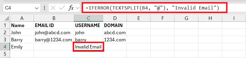
In this arrangement:

• A2 to A4 contains the email address you’re looking to split.
• "@" is the delimiter upon which the split is based, as email addresses typically have a username followed by “@” and the domain.
• The fourth argument TRUE indicates that the split should be oriented across columns.
• The IFERROR function envelops this TEXTSPLIT formula to effectively check for and manage any errors during the split.
• "Invalid Email" is the message that will be presented in lieu of an error if TEXTSPLIT encounters a problem, such as when the cell is empty.

By doing so, you elegantly handle potential problems and substitute the error with a meaningful placeholder. This ensures that your dataset remains interpretable and that subsequent analysis or sorting based on the split data isn’t compromised.

 

Frequently Asked Questions

How do I use Iferror in Excel?

To use the IFERROR function in Excel, start by clicking on the cell where you want the result to appear, then type the following formula in the cell –

=IFERROR(value, value_if_error)

In this formula, replace ‘value’ with the cell reference or formula you’re evaluating for errors, and ‘value_if_error’ with the output you want if an error is detected. Once you’ve entered the formula, press “ENTER,” and Excel will display either the error-free result of ‘value’ or the specified ‘value_if_error’ if an error is found.

How do you get the formula if error show 0 in Excel?

To ensure a formula in Excel displays a 0 instead of an error, you can use the `IFERROR` function by structuring the formula like this: `=IFERROR(your_formula,0)`. This will return 0 if the formula results in any error, including the #DIV/0! error. For example, if your formula is `=A2/A3`, you would write `=IFERROR(A2/A3,0)`.

What is the difference between Ifna and Iferror in Excel?

The difference between IFNA and IFERROR in Excel lies in their scope and specificity for handling errors. IFNA is designed to catch and handle only the #N/A errors, typically arising from lookup functions when a value is not found, while IFERROR is a broader error-handling function that captures and handles all types of errors within a formula, potentially masking various issues unless a unified response is desired.

How does IFERROR differ from other error handling functions?

The IFERROR function in Excel not only identifies errors within a formula but also allows users to specify an alternative value to display instead of the error. This differs from other error-handling functions like ISERROR, which only report if an error exists by returning a True or False value, without offering the option to replace the error with a custom output. Consequently, IFERROR provides a more dynamic solution by both detecting errors and managing their presentation directly within the formula itself.