Summarize Data With Dynamic Subtotals

Working with data in Excel often feels like trying to keep a dozen spinning plates in the air. Between raw numbers, multiple categories, and ever-changing inputs, I’ve had my fair share of spreadsheet-induced headaches. One trick that’s helped me slice through the chaos? Dynamic Subtotals.

If you’ve ever been frustrated by static summaries or needed to adjust totals on the fly based on filters or data changes, you’re going to love what I’m about to share. I’m going to walk you through how to summarize data with dynamic subtotals in Excel, when to use them, what to watch out for, and how to harness their power truly.

Key Takeaways:

• Dynamically summarize data using the SUBTOTAL function and a combo box for instant, flexible analysis without additional formulas.
• The combo box’s cell link powers dynamic calculations by providing the right function_num for SUBTOTAL based on user selection.
• Align your summary list and function numbers using a helper list or named range to ensure accuracy and ease of use.
• This approach keeps dashboards clean and professional, even as the analytic depth and interactivity increase.
• Empower users to analyze key metrics themselves by presenting clear interactive controls, enhancing engagement and insight.

Download excel workbookSubtotal-Dynamically.xlsx

Understanding Subtotals: More Than Just a Total

What Is a Subtotal in Excel?

At its core, the SUBTOTAL function allows me to perform a range of calculations—such as SUM, AVERAGE, COUNT, MAX, MIN, and more—on data that remains dynamic, especially when filtered or grouped. Unlike traditional functions like SUM or AVERAGE, SUBTOTAL only includes visible data, which means that if I filter my data, the function automatically updates to reflect my selection. This flexibility is critical when I want to explore different segments of my dataset without rewriting formulas each time.

What does it do?

It returns a Subtotal in a list or database

Formula breakdown:

=SUBTOTAL(function_num, ref1)

What it means:

=SUBTOTAL(function number 1-11 includes manually-hidden rows & 101-111 excludes them, your list or range of data)

Why Subtotals Matter in Real Life

When I first began handling spreadsheets with hundreds or even thousands of records, it quickly became apparent that simple sums or averages weren’t enough. I needed a way to see breakdowns—like sales by region or expenses by category—without resorting to multiple filtered views or separate sheets.

That’s when I stumbled upon the Subtotal feature in Excel. It didn’t just aggregate data—it let me dynamically adjust and analyze my data on the fly, drilling down or rolling up as needed. I could see not just the grand total, but the story behind the numbers. The beauty of subtotals is their ability to adapt to how the data is structured, providing immediate, meaningful insights without having to write complex formulas.

Steps to Summarize Data with Dynamic Subtotals

The Subtotal function can become dynamic when we combine it with a drop-down list. This is a great trick and one that can be used when creating an Excel Dashboard that summarizes key data metrics on one page.

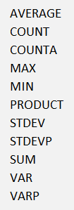
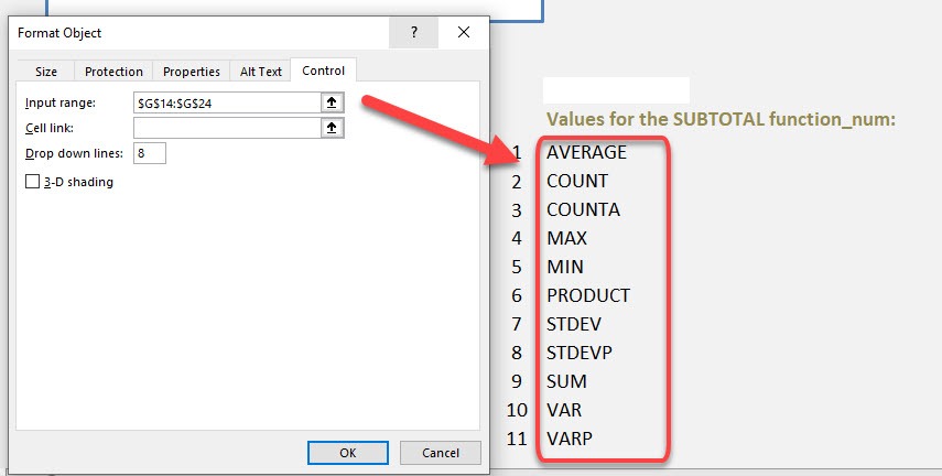
STEP 1:  We need to list the Subtotal summary functions in our Excel worksheet

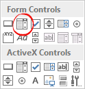
STEP 2: In the ribbon select Developer > Insert > Form Controls > Combo Box

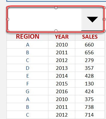
STEP 3: With your mouse select the region where you want to insert the Combo Box

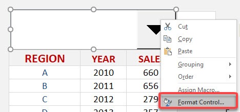
STEP 4: Right Click on the Combo Box and select Format Control…

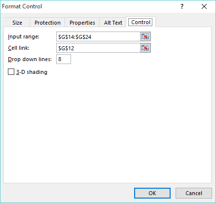
STEP 5: For the Input Range, you need to select the range with the Subtotal summary names from STEP 1

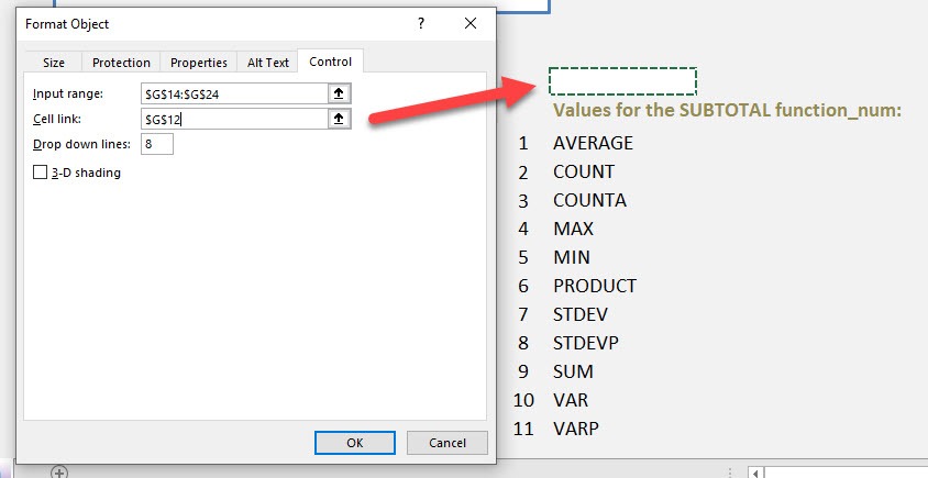
STEP 6: For the Cell Link, you need to select a cell where you want to show the output and press OK

(The Cell Link increments by 1 depending on the order of the list and the name chosen.  We will use this value as our first argument in the SUBTOTAL function)

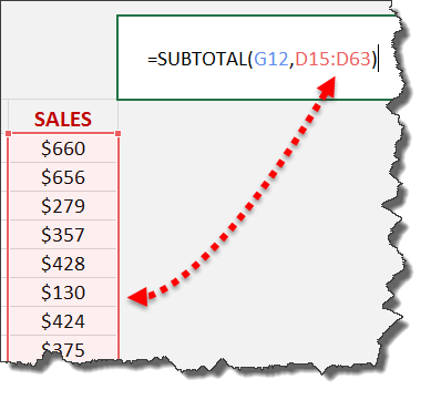
STEP 7: Enter the Subtotal function and for the first argument function_num we will reference the Cell Link from STEP 6

STEP 8: For the second argument, select the data range

So you can see as you choose a summary name from the drop-down list, it gives us a value for the Cell Link, which is equal to the function_num for that summary name!

 

Tips & Tricks

Exploring SUBTOTAL Function Numbers

One sub-topic that often confuses beginners is what the SUBTOTAL function numbers actually mean. Each number between 1 and 11 and 101 to 111 corresponds to a different summary operation—like 1 for AVERAGE, 2 for COUNT, 9 for SUM, and so on. The numbers above 100 ignore hidden rows, which is particularly useful when you want summaries that adapt to filtering. I keep a reference table handy in my dashboard to clarify which number does what, making it easier to expand or adjust summary types later on.

 

SUBTOTAL vs. Other Aggregation Functions

Another important sub-topic is how SUBTOTAL compares to other Excel aggregation functions like SUM, AVERAGE, or COUNT. The key advantage of SUBTOTAL is its ability to aggregate only visible rows, which is invaluable when data is filtered. Whereas SUM or AVERAGE will always calculate on the entire range, SUBTOTAL adapts to the view, ensuring dynamic accuracy. This makes it my preferred choice for interactive dashboards or anytime I anticipate users applying filters to the dataset.

 

FAQs

1. What advantages does this combo box and SUBTOTAL method offer over traditional summary cells?

Using a combo box with the SUBTOTAL function means my worksheet doesn’t get cluttered with separate summary cells for each possible calculation. It also lets me (and my colleagues) switch summary types instantly, without the need to rewrite formulas or create multiple reports. Maintenance becomes much easier, and the dashboard remains visually appealing and simple to navigate, regardless of how much data we’re summarizing.

2. How do I ensure the drop-down list matches the correct SUBTOTAL function numbers?

To keep everything accurate, I use a helper column or named range to store the official SUBTOTAL function numbers (like 1 for AVERAGE, 2 for COUNT, 9 for SUM, etc.). I make sure the order of functions in my drop-down matches the list, and then use the INDEX function to retrieve the right function number based on the drop-down’s output. This linkage is the key to error-free, dynamic summaries that always show what users expect.

3. Does this method work if I filter my data in Excel?

Yes! One of the best features of the SUBTOTAL function is its ability to operate on visible (filtered) rows only. When I filter my data—say, to see results for a specific region or manager—the SUBTOTAL formula automatically recalculates to reflect just the filtered subset. This makes the combo box + SUBTOTAL approach perfect for interactive dashboards and ad hoc queries where data visibility changes frequently.

4. Can I adapt this technique for multiple metrics or even multiple data sets?

Absolutely. I often build dashboards with several combo boxes, each linked to a different metric (sales, expenses, profit, etc.), and each controlling its own dynamic SUBTOTAL formula. You can expand this setup to suit any number of key metrics or even different data ranges within the same sheet. It’s scalable, flexible, and ensures your dashboards can grow alongside your reporting needs.

5. How can I make my dynamic subtotal dashboard user-friendly for people unfamiliar with Excel?

I find that clear labels, brief instructions, and consistent formatting make the biggest difference. I usually include a short note explaining how to use the drop-down, highlight the summary cell with a bold border or color, and keep the controls grouped logically. Sometimes, I use data validation to restrict input or add error messages for extra clarity. The end goal is always to make the dashboard as intuitive and self-explanatory as possible.