Timeline Slicers In Microsoft Excel

Excel is a powerhouse for managing and analyzing data, but many users still rely on basic dropdown filters in Pivot Tables. Timeline Slicers take filtering to the next level—built specifically for dates, they let you scroll through months, quarters, or years with a simple drag and watch your Pivot Table update instantly.

Got a Pivot Table with dates? Add a Timeline Slicer and dynamically filter your data in seconds—you’ll be amazed at what it can do!

In this guide, we’ll show what Timeline Slicers are and why they’re game-changing.

Key Takeaways:

• Timeline Slicers allow you to filter Pivot Table data by date ranges interactively.
• They are easier to use and more visual than standard slicers.
• You can filter by different time units like days, months, quarters, or years.
• Timeline Slicers update your Pivot Table instantly with a simple drag.
• Creating one only takes a few clicks in Excel.

 

What Are Timeline Slicers?

Definition and Purpose

Timeline Slicers are a special type of Excel slicer created exclusively for fields formatted as dates. Unlike standard slicers that show lists of categories, Timeline Slicers display time periods in a slider format that you can move, stretch, or shrink to adjust the filtered data.

The main purpose of a Timeline Slicer is to make it easier for users to interact with data involving time, such as sales orders, employee attendance, financial reports, or project deadlines. Instead of manually selecting multiple months from a dropdown, you simply drag a bar to cover the period you want to analyze.

How They Differ from Normal Slicers

While normal slicers let you filter by categories (like Region, Product, or Department), Timeline Slicers are designed specifically for date hierarchies. This difference matters because a regular slicer would list each date as an item, making it nearly impossible to navigate large datasets. With a Timeline Slicer, Excel automatically groups dates into manageable time units—days, months, quarters, and years—making filtering intuitive and fast.

 

How to Insert Timeline Slicer

Creating the Pivot Table

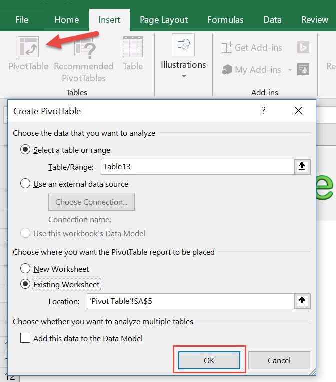
STEP 1: Insert a new Pivot table by clicking on your data and going to Insert > Pivot Table > New Worksheet or Existing Worksheet

 

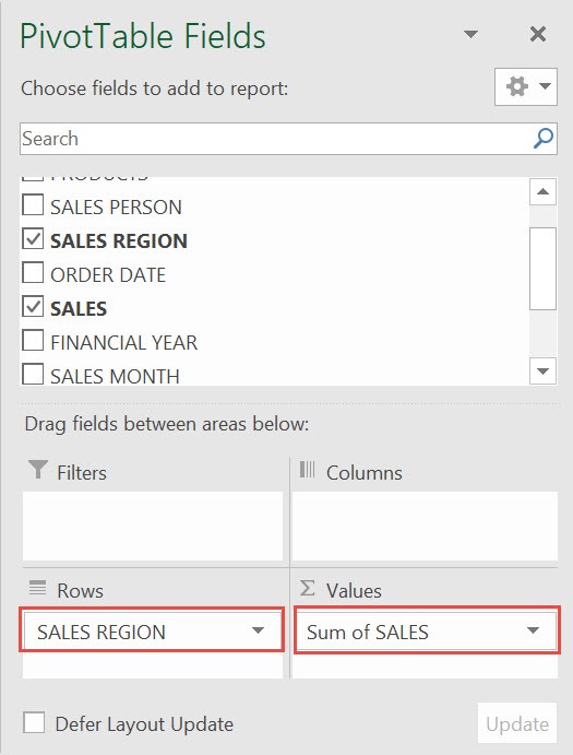
STEP 2: In the ROWS section put in the Sales Region field.  In the VALUES section put in the Sales field.

Adding the Timeline Slicer

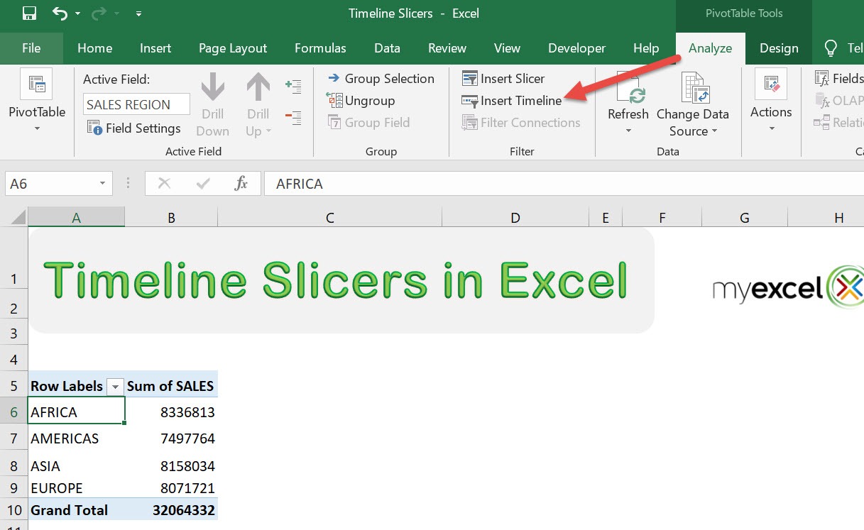
STEP 1: Let us now add our timeline slicer! Go to PivotTable Tools> Analyze > Filter > Insert Timeline

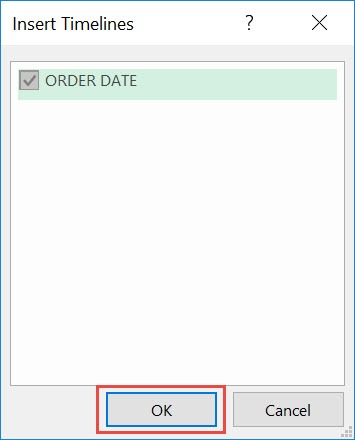
STEP 2: Make sure ORDER DATE is ticked. Click OK.

 

And now you have your Timeline Slicer! You can play around and set different date ranges, then the pivot table data will also adjust accordingly.

See this example where we tried Jan 2012 – Mar 2012. You can also change the unit (e.g. months, years, etc.) of your slicer!

 

Practical Uses of Timeline Slicers

Timeline Slicers are more than just a neat Excel trick—they bring real analytical power to your reports. Here are the different applications of Timeline Slicers –

• Sales teams can use Timeline Slicers to track revenue by months, quarters, or years.
• Finance departments can filter expense and budget data by fiscal periods.
• Project managers can monitor task progress across weeks or specific milestones.
• Inventory teams can analyze stock movement trends by season or year.
• Marketing teams can evaluate campaign performance based on the campaign duration.
• HR departments can review employee attendance and leave records over tim

 

Troubleshooting and Best Practices

Common Issues

• Date Field Not Available: If you don’t see your date field when inserting a Timeline, check whether the column is formatted as a date in Excel.
• Empty Slicer: If the slicer shows blank or doesn’t filter properly, ensure your Pivot Table is built from a properly formatted source.

Best Practices for Smooth Use

• Always clean and format your date columns before creating a Pivot Table.
• Avoid mixing text and date values in the same column.
• Use clear labels in your Pivot Table so the effect of the Timeline Slicer is obvious to others viewing your report.

 

FAQs

1. What is a Timeline Slicer in Excel?

A Timeline Slicer is a special filtering tool in Excel designed specifically for date fields in Pivot Tables. Unlike normal slicers that display categories, Timeline Slicers show dates in a visual slider format. This makes it easy to filter data by days, months, quarters, or years with a simple drag. The key advantage is speed—you don’t have to scroll through long dropdown lists. Instead, you just adjust the slider and watch your Pivot Table update instantly.

2. How do I insert a Timeline Slicer into a Pivot Table?

To insert a Timeline Slicer, first create a Pivot Table that includes a date field such as “Order Date.” Then go to PivotTable Tools > Analyze > Filter > Insert Timeline. Select the date field you want, click OK, and the slicer will appear next to your Pivot Table. You can now drag across the timeline to filter data by specific periods. It only takes a few clicks to set up and immediately makes your data more interactive.

3. What are the main benefits of using Timeline Slicers?

Timeline Slicers make it simple to filter large datasets by time periods without scrolling through endless lists. They let you instantly adjust between different levels like days, months, quarters, and years. This makes your reports much more flexible and easier to explore. They also provide a visual, interactive experience, which helps non-technical users understand trends quickly. In short, they save time, reduce complexity, and make your Pivot Tables more powerful.

4. Can I use Timeline Slicers along with normal slicers?

Yes, Timeline Slicers can work seamlessly with standard slicers. For example, you could use a normal slicer to filter by Region and a Timeline Slicer to filter by Year at the same time. This combination creates layered filtering that’s easy to manage and very effective for analysis. It allows you to drill down into specific data subsets quickly. Together, they provide both categorical and time-based filtering for your reports.

5. What should I do if my Timeline Slicer doesn’t work?

If your Timeline Slicer isn’t working, the most common issue is that your date field isn’t formatted properly. Make sure your date column in the source data is stored as a valid date, not text. If the slicer appears blank, check that your Pivot Table is linked to clean, consistent data. Also avoid mixing text and date values in the same column. Once your data is properly formatted, the Timeline Slicer should work smoothly.