Vlookup in an Excel Table

Excel Tables are just amazing and should be used all the time, whether you have 2 rows or 200,000 rows of data! When you use a Vlookup formula to lookup in an Excel Table then your formula becomes dynamic due to its structured referencing. What that means is that as the Excel Table expands with more data added to it, your Vlookup formula’s 2nd argument (table_array) does not need to be updated as it refers to the Excel Table as a whole by referring to its name eg Table1  or Table2  or Table3  etc. In the example below our Excel Table name is Table2 and as we add more rows of data to it, the Vlookup formula does not need to be adjusted.  How cool is that?

You can read the benefits of using an Excel Table here: Excel Tables

Key Takeaways

• VLOOKUP Function for Table Lookup – VLOOKUP is commonly used to search for a value in the first column of a table and return a value from another column in the same row.
• Absolute vs. Relative References – When using VLOOKUP in tables, ensure that the table array is referenced absolutely (e.g., $A$2:$D$10) to prevent errors when copying the formula across cells.
• Column Index for Data Retrieval – The column index number determines which column’s data VLOOKUP will return. The first column is always 1, the second is 2, and so on.
• Exact and Approximate Match – By default, VLOOKUP performs an approximate match. To get an exact match, set the last argument to FALSE.
• Table References with Structured References – When using VLOOKUP with tables, use structured references like TableName[ColumnName] for more readable formulas instead of cell references.

Quick Overview

What does it do?

Searches for a value in the first column of a table array and returns a value in the same row from another column (to the right) in the table array.

Formula breakdown:

=VLOOKUP(lookup_value, table_array, col_index_num, [range_lookup])

What it means:

=VLOOKUP(this value, TableName, and get me value in this column, Exact Match/FALSE/0])

How to Use Vlookup in an Excel Table

STEP 1: We need to convert the data into an Excel Table. Press Ctrl + T then press OK.

STEP 2: Now let us create the formula to get the price of the Laptop. Let us use the VLOOKUP formula:

=VLOOKUP(G15, Table1, 2, FALSE)

This will get the lookup value (Laptop in Cell G15), then search in the first column of Table1.

Afterwards it will get the value in Column #2 which is the price. The FALSE means is we want to get the exact match.

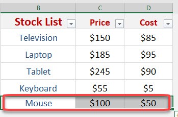
STEP 3: Drag down the formula to copy it across the table. Notice that the second row is looking for the price of Mouse. This does not exist in our data table yet.

STEP 4: Now add and type in a new row in our table for the price of the mouse.

The beauty with this is our VLOOKUP formula still works fine. Since we are using the Table1, there is no need to update the range of values that our VLOOKUP will use. It is now automatically included and the price of the mouse is retrieved right away.

Frequently Asked Questions

What is the purpose of the VLOOKUP function in Excel?

VLOOKUP is used to look up a value in the first column of a table and return a corresponding value from another column in the same row, making it useful for data retrieval and matching.

How do I prevent errors when copying VLOOKUP formulas across cells?

Use absolute references (e.g., $A$2:$D$10) for the table array to ensure that the range doesn’t shift when you copy the formula to other cells.

How does the column index number work in the VLOOKUP formula?

The column index is the number of the column within the table from which you want to retrieve data. The first column is 1, the second is 2, and so on.

What’s the difference between an approximate match and an exact match in VLOOKUP?

An approximate match (default) looks for the closest value below the lookup value, while an exact match (set by using FALSE as the last argument) requires an exact match.

How can I use VLOOKUP with an Excel Table instead of cell references?

Use structured references in your VLOOKUP formula like TableName[ColumnName], which makes the formula easier to read and less prone to errors compared to using traditional cell references.