Different Ways to Filter an Excel Slicer

Slicers are an interactive, visual way to filter your PivotTables and PivotCharts. Unlike old-school dropdown filters that are buried in menus, Slicers bring a sleek, button-style interface right into your spreadsheet, making your dashboards not only easier to use—but also way more intuitive and visually appealing. Think of them as on-screen remotes for your PivotTables. You click a button, and boom—the data updates instantly. Plus, Slicers show you exactly what’s selected. No more guessing what’s been filtered!

In this article, we’ll walk you through several different ways to filter an Excel Slicer, and we’ll include both keyboard and mouse tricks to speed things up.

Key Takeaways:

• Slicers provide a clear and interactive way to filter data in PivotTables and PivotCharts.
• You can use your mouse or keyboard shortcuts like CTRL and SHIFT to filter multiple items.
• Their button-style design makes slicers ideal for dashboards and easy for anyone to use.
• The Clear Filter button lets you instantly reset all filters to view full data again.
• When linked to multiple PivotTables, slicers keep your reports consistent and easy to control.

 

 

Understanding Excel Slicers and Their Benefits

What Is an Excel Slicer?

Before diving into the different ways to use Slicers, it’s important to understand what they are. An Excel Slicer is a visual, interactive tool that allows you to filter data within PivotTables, PivotCharts, Excel Tables, and even Power Pivot models. It appears as a floating box with a list of items—such as regions, categories, or products—displayed as clickable buttons. By selecting or deselecting these buttons, you can instantly apply or remove filters from your data.

Why Use a Slicer?

Slicers are a powerful upgrade from traditional filter drop-downs, and here’s why they’re worth using:

• They offer a clear visual representation of which filters are currently applied, making it easy to understand your data at a glance.
• You can select multiple items quickly using mouse or keyboard shortcuts, without needing to scroll through menus.
• Slicers are particularly useful in dashboards, as they provide a clean and user-friendly interface for end users.
• Any changes you make using a Slicer update the data in real time, allowing for faster insights and more interactive reports.

Whether you’re preparing a sales dashboard, summarizing financial data, or analyzing trends, Slicers help make your Excel reports more dynamic and engaging.

Different Ways to Filter an Excel Slicer

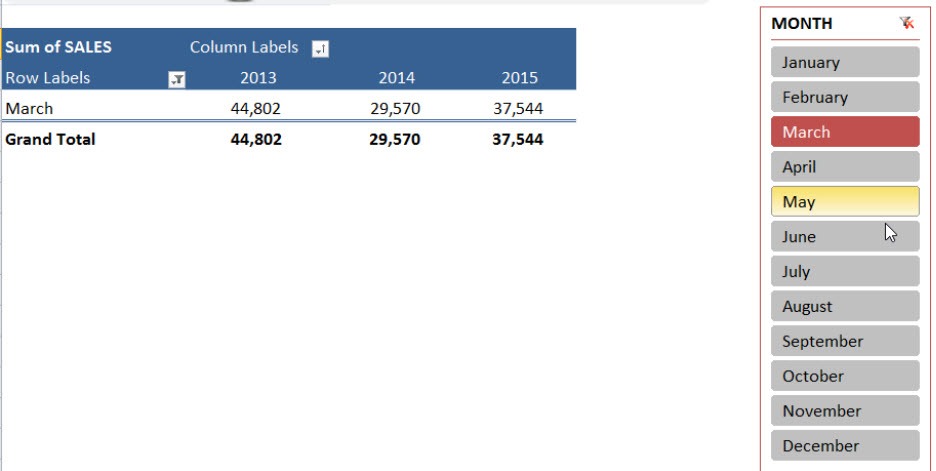
Clicking with your left mouse button is the most direct way to filter a Slicer.

How it works:

• Click on a Slicer item with your left mouse button.
• The PivotTable updates immediately to show only that selected item.

This method is perfect for single selections—fast, easy, and intuitive.

DRAG LEFT MOUSE BUTTON:

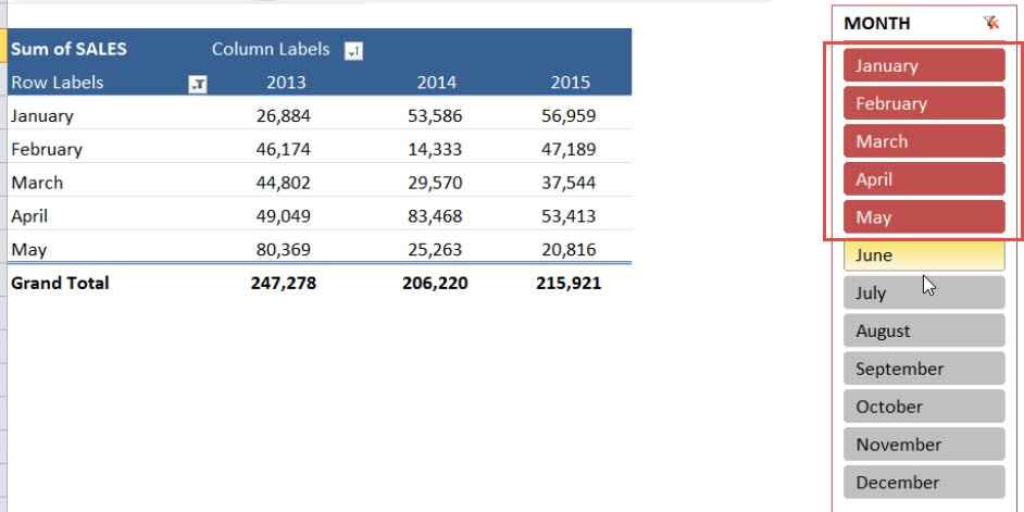
You don’t have to click one by one if the items are adjacent. Use the click + drag technique.

How it works:

• Click on the first item with the left mouse button.
• Hold the button down.
• Drag down or up to select a consecutive range of items.

This trick is ideal when you want to quickly filter, say, “January” through “June” in a month slicer.

CTRL KEYBOARD:

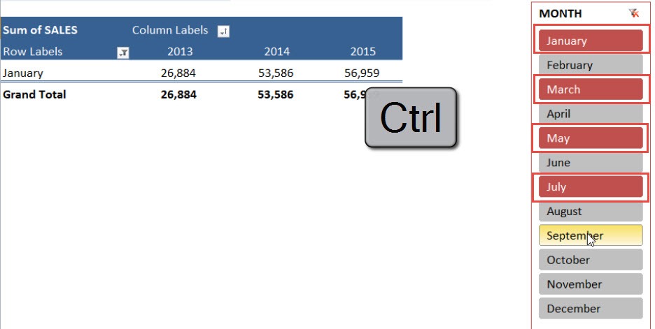
Need to select “January”, “March”, and “May” but skip the rest? No problem.

How it works:

• Hold down the CTRL key on your keyboard.
• Then, click on the items you want using your left mouse button.

You can pick and choose any combination you like—no need for them to be next to each other.

SHIFT KEYBOARD:

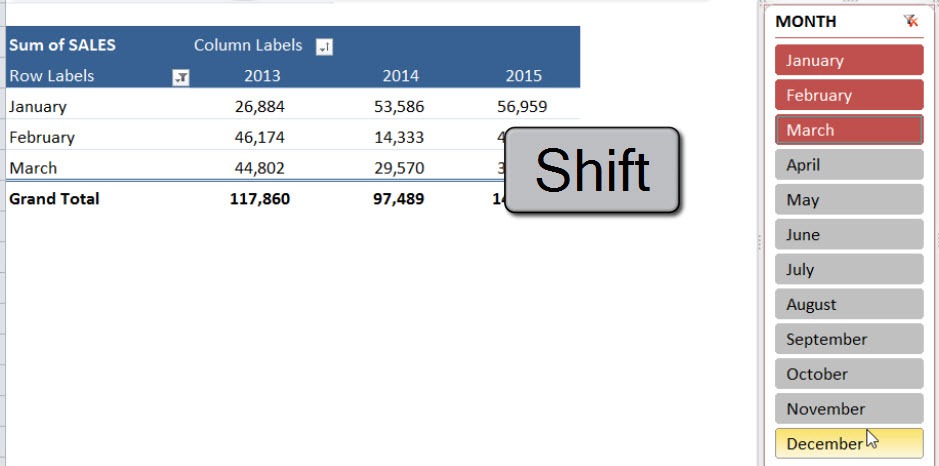
This one’s a game-changer when dealing with a long list.

How it works:

• Click on the first Slicer item you want.
• Hold down the SHIFT key.
• Click on the last item in the range.

Excel will automatically select everything in between—much faster than dragging across 50 items!

CLEAR FILTER BUTTON

Sometimes, you just want to remove all filters and start fresh.

How it works:

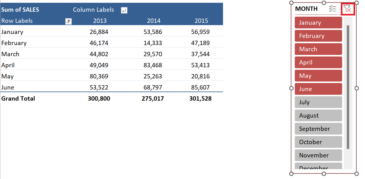
• Look at the top-right corner of the Slicer box.
• You’ll see a small filter icon with a red ‘X’.
• Click it to clear all selections.

Your PivotTable goes back to showing everything, like a factory reset for your filter.

 

Common Mistakes to Avoid

• Selecting multiple slicer items without using CTRL or SHIFT – Clicking multiple buttons without holding CTRL or SHIFT will reset your selection. It’s a classic slip-up.
• Forgetting to clear filters – Your PivotTable looks empty? You might still have filters applied. Always double-check and use the Clear Filter button.
• Not connecting slicers to multiple PivotTables – If one table updates and the others don’t, it’s likely you forgot to link the slicer to all data sources.

 

FAQs

1. What’s the difference between a slicer and a regular filter in Excel?

A regular filter is typically applied through drop-down menus at the top of a column or PivotTable field. It works fine but lacks visibility—users can’t always tell what’s filtered at a glance. An Excel slicer, on the other hand, is a floating box with clearly labeled buttons that visually show what is currently selected. It makes interacting with the data faster and more intuitive, especially in dashboards or presentations.

2. Can I use slicers with multiple PivotTables or charts at the same time?

Yes, you can connect a single slicer to multiple PivotTables and PivotCharts—as long as they share the same data source. To do this, click on the slicer, go to the Slicer Tools > Options tab, and click Report Connections (or “PivotTable Connections”). From there, you can select which PivotTables the slicer should control. This makes your report more cohesive and ensures consistent filtering across different views of the data.

3. Why does my slicer only affect one PivotTable even though I have multiple in the sheet?

The slicer may not be connected to all the PivotTables you want it to control. Excel doesn’t automatically link slicers to multiple tables—you have to do it manually through the Report Connections dialog box. Also, make sure all PivotTables are based on the same data source; slicers can’t control tables based on separate datasets. Once connected properly, changes made in the slicer will reflect across all selected PivotTables.

4. How can I select multiple items in a slicer efficiently?

To select multiple items that are adjacent, click and drag with your left mouse button. For non-adjacent items, hold down the CTRL key and click each item you want. If you want to select a range, click the first item, hold down SHIFT, then click the last item. These shortcuts save time and give you more control when filtering large sets of slicer items.

5. What should I do if my PivotTable shows no data after using a slicer?

This usually means the slicer is filtering your data down to a set that has no matching records. First, check if multiple slicers are applied at the same time, as their combined filters might exclude all results. If needed, use the Clear Filter button (the small filter icon with a red ‘X’ in the top-right corner of the slicer) to reset the selections. Always double-check that your slicer filters are set to include relevant data points.