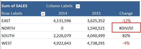
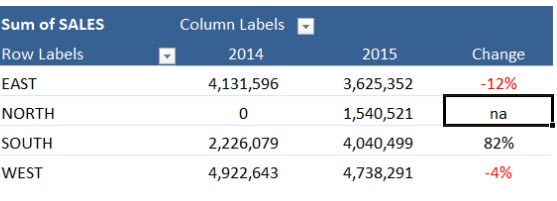
Whenever you do a calculation in an Excel Pivot Table you may get an error value like a #DIV/0!
This looks ugly when you are presenting important information. Luckily you can override this with a custom value or text.
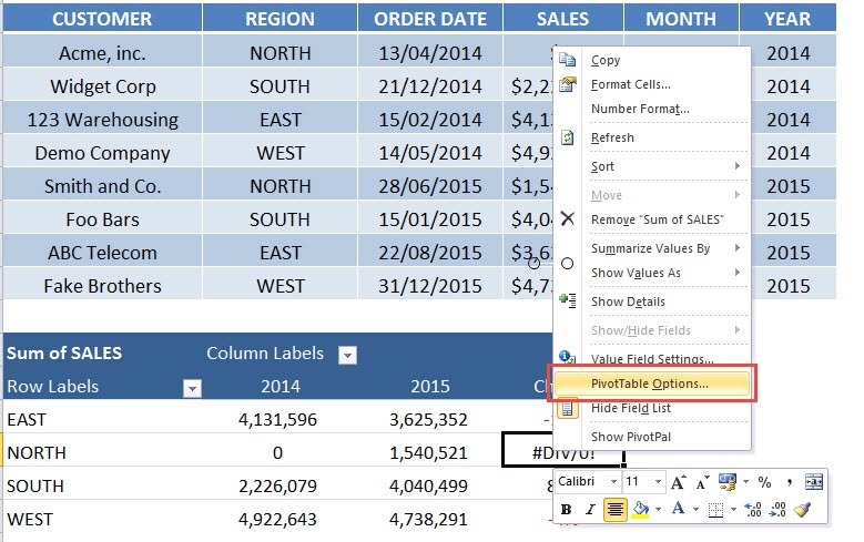
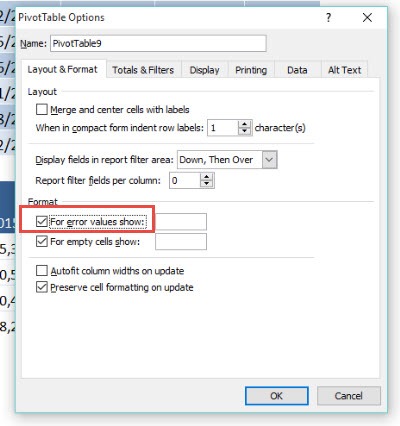
To activate this you need to Right Click in any Value in your Excel Pivot Table and choose PivotTable Options and “Check” the box that says: For error values show
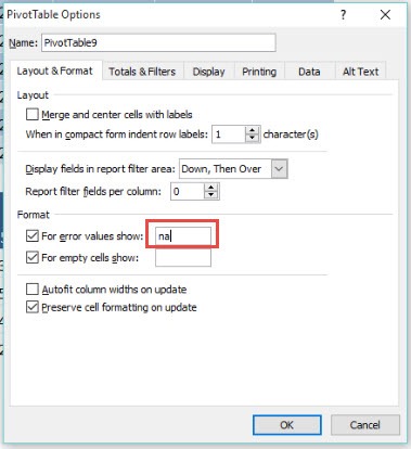
This activates the box and you can now enter any value or text that you want to show whenever your calculation has an error.
STEP 1: We have an error in the pivot table calculation.
STEP 2: Right click on any value and Go to Pivot Table Options.
STEP 3: Check the Box: For Error Values Show
STEP 4: Enter any text or value
Now your error values are properly formatted!
John Michaloudis is a former accountant and finance analyst at General Electric, a Microsoft MVP since 2020, an Amazon #1 bestselling author of 4 Microsoft Excel books and teacher of Microsoft Excel & Office over at his flagship MyExcelOnline Academy Online Course.


