How to get Remainder in Excel using MOD Formula

In Excel, it is very easy to divide two numbers. But how about if you need to get the remainder from a division operation? Thankfully we can do the above complex and manual calculation with ease using Excel’s MOD formula!

Key Takeaways

• To calculate a remainder in Excel, you can use the MOD function, which is designed to return the remainder after dividing one number by another. The function is implemented by typing ‘=MOD(number, divisor)’ into a cell, where number is the value you want to divide and divisor is the number you are dividing by.
• It’s essential to perform a double-check of the results when using the MOD function to ensure accuracy. While the function is straightforward, mistakes can happen, especially with complex spreadsheets or data sets. Verifying your calculations can prevent potential errors in your analysis or reporting.
• Understanding how to use the MOD function is beneficial for various data analysis tasks that require remainder calculations. This function simplifies what would otherwise be a manual and time-consuming process, allowing you to perform this operation with ease and integrate it seamlessly into larger analytical processes within Excel.

MOD Function – Syntax & Basic Use

What does it do?

Gives you the remainder after dividing one number with another

Formula breakdown:

=MOD(number1, number2)

What it means:

• number1 – A number whose remainder you wish to find.
• number2 – A number to divide with.

For example, divide 13 by 4:

• Divide the two numbers (i.e. 13 / 4)
• Get the quotient (which is 3)
• Multiply it back to the divisor (3 * 4)
• Subtract it from the original number (13 – 12)
• And I have the remainder! (1)

So, 4 goes into 13 three times with a remainder of 1.

So, MOD(13,3) returns 1 as when you divide 13 by 3 will give a quotient of 4 and leaves a remainder of 1.

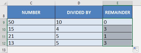
Let’s look at a few examples to know how to get remainder in Excel using the MOD formula.

 

STEP 1: We need to enter the MOD function:

=MOD(

 

STEP 2: The MOD arguments:

number1

What is the first number that we plan to divide?

Reference the cell that contains the first number:

=MOD(C9,

number2

What is the divisor?

Reference the cell that contains the second number:

=MOD(C9, D9)

STEP 3: Do the same for the rest of the cells by dragging the MOD formula all the way down using the left mouse button.

Now you are able to get the remainders of all the division operations!

Now that you have learned how to use the MOD function to find the remainder. Let’s move on to some practical uses of this function.

 

Use MOD function to Highlight Cells

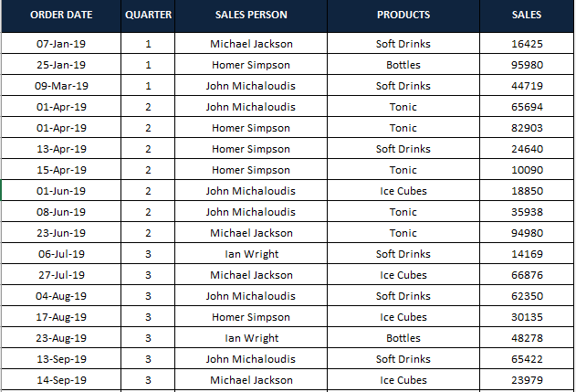
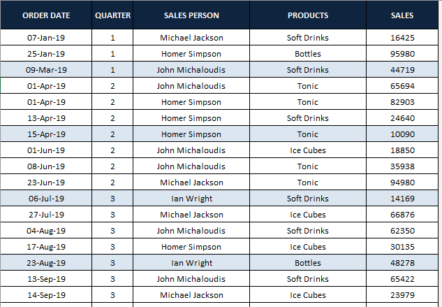
You can use the MOD function to conditionally format the cells. Say, you want to highlight every 4th row in your data.

Let’s see the data table below:

 

Let’s follow the step-by-step tutorial below to highlight every 4th row of this data table:

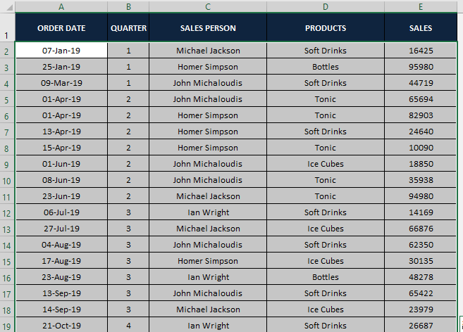
STEP 1: Select the entire data table.

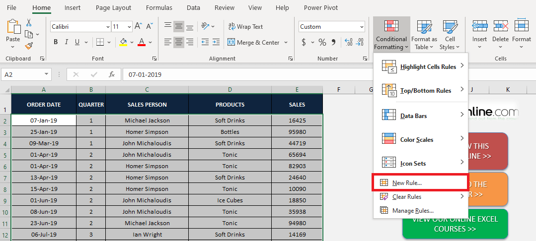
STEP 2: Go to Home > Conditional Formatting > New Rule.

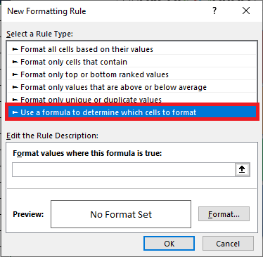
STEP 2: In the New Formatting dialog box, select Use a formula to determine which cells to format from the list.

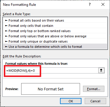
STEP 4: Type the formula

=MOD(ROW(),4)=0

under Format values where this formula is true text box, and then click on Format button to apply custom formatting to these rows.

Using this formula you can add formatting to every 4th row of the data. You can change the number to 2,3,5… as per your need.

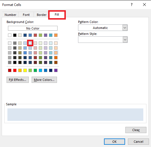
STEP 5: In the Format Cells dialog box, Go to Fill Tab, and select an appropriate color. Click OK.

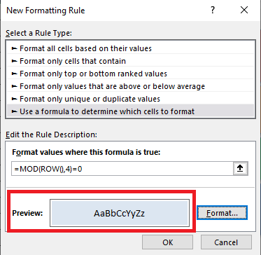
STEP 6: Here you can see a preview of how your formatted data will look like. If you are satisfied with it, click OK.

 

Your conditionally formatted data table using the MOD formula is now ready!

To highlight, the n^th column you can simply replace the ROW formula with the COLUMN formula.

This conditional formatting is dynamic, i.e. once you add or delete more rows the formatting will update automatically.

As you have seen, you can use the MOD function to highlight the nth row or column of your data. You can also use it to sum every nth row/column.

 

Use MOD function to Calculate cells

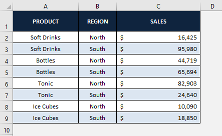
In the data below, you have sales data for different products & different regions.

You can use the MOD function, to sum up, every alternate row in the data to get the total sales of the North and South regions separately.

 

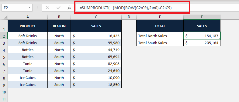
The formula for the sum of every even row (North Region Sales) :

=SUMPRODUCT(- -(MOD(ROW(range),2)=0),range)

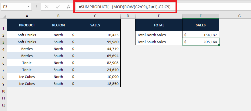
The formula for the sum of every odd row (South Region Sales) :

=SUMPRODUCT(- -(MOD(ROW(range),2)=1),range)

Here,

• The ROW function returns the row number of the cell.
• MOD function when divides an even number leaves remainder as 0 and when divides an odd number leaves remainder as 1.
• Double dashes (- -) outside the MOD function converts the FALSE and TRUE into 0s and 1s.
• Lastly, SUMPRODUCT function multiplies the sum of the product of range containing 0s and 1s and range containing sales amount.

 

The formula for calculating total sales in North Region i.e., the summation of all even rows (Row 2, Row 4, Row 6 & Row 8) will be:

 

The formula for calculating total sales in South Region i.e., the summation of all odd rows (Row 3, Row 5, Row 7 & Row 9)  will be:

Advanced Techniques for Excel Enthusiasts

Dynamically Highlighting Rows and Columns

Dynamically highlighting rows and columns in Excel doesn’t have to be a mundane task—thanks to the MOD function, it becomes an effortlessly dynamic endeavor. With just a few clicks, you can apply custom highlights that clearly define certain rows or columns based on specific intervals, making your data far easier to navigate and analyze.

Whether you’re a financial analyst looking to accentuate every fifth row to delineate weekly data, or a project manager aiming to highlight every third column to signify quarterly milestones, MOD is your go-to ally. Simply use the MOD function within conditional formatting to set up rules that bring your cells to life.

The process is straightforward:

• Select the range you wish to format.
• Create a new conditional formatting rule using the formula =MOD(ROW(), n) = 0 for rows or =MOD(COLUMN(), n) = 0 for columns, where n is the interval at which you want the highlight to occur.
• Choose a fill color and apply the formatting.

Voilà! Your data now pops with intelligently spaced highlights that not only please the eye but also serve a functional purpose. As your worksheet grows or shrinks, the highlights adapt, maintaining your insights and keeping the flow of information crisp and clear.

Get ready to say goodbye to manual cell-by-cell formatting and embrace the power of automation with MOD—a true game-changer in data presentation.

Complex Calculations Simplified

When it comes to more intricate computations, the MOD function in Excel can uncomplicate the seemingly complicated. Whether you’re dealing with financial models, engineering equations, or statistical analysis, MOD can help you simplify these calculations by dealing with periodicity and cycles efficiently.

Imagine you’re an engineer calculating load cycles or a finance professional analyzing investment periods. You could be facing a daunting task made up of endless repetition and complexity. Here, MOD steps in as your silent mathematician, proficiently handling these repetitive cycles, leaving you with the core data you need to make informed decisions.

For example, to calculate regular payment intervals or periodic investments, the MOD function can be used to identify specific payment periods within a larger cycle. It can effortlessly segment a set of data into regular intervals, turning a mountain of calculations into manageable and meaningful outcomes.

Moreover, in probabilistic models or game theory, where outcomes are often evaluated based on various stages or turns, MOD can identify and group these stages. Thus, it simplifies pattern recognition and strategy development.

By embracing MOD as your complex calculation ally, you ensure that the heavy lifting in your Excel workbooks is done neatly, efficiently, and with fewer opportunities for manual error.

Navigating Common Hurdles

Troubleshooting MOD Function Pitfalls

While the MOD function in Excel is straightforward, it isn’t immune to mishaps, which can lead to inaccuracies or errors. To stay on the safer side of spreadsheet sorcery, it’s essential to recognize where things can go awry and how to address them.

One common hiccup occurs with incorrect formula entry. Keep an eye out for typos or syntax issues that cause errors such as #NAME or #VALUE. These usually signal that Excel doesn’t recognize the input, possibly due to misspelled functions or invalid argument types.

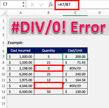
Another pitfall is the infamous #DIV/0! error. This pops up when the divisor in your MOD function is zero—after all, dividing by zero is one of math’s cardinal sins. Always ensure your divisor is a non-zero number to keep your formulas error-free.

Remember to use absolute and relative cell references appropriately. A mix-up here can easily lead to a spreadsheet that confuses rather than clarifies. For example, when applying MOD across multiple cells, ensure that the divisor remains constant if needed by making it an absolute reference (with $ signs).

Finally, consider the data type you’re working with. MOD handles numbers, but what about text or dates? Ensure to convert your data into a compatible format when necessary before running the MOD calculation.

Ensuring Accuracy with Error Detection

Accuracy is paramount in Excel, and this is where the MOD function can play a critical role in error detection. It works like a charm when it comes to spotting inconsistencies within your datasets, especially when dealing with periodic or cyclical data.

To ensure your calculations don’t lead you astray, double-check your datasets before applying the MOD formula. Accurate input data is a must as even the most sophisticated formulas can’t compensate for erroneous or misrepresented figures. Verification may involve scanning for outliers, ensuring data consistency across cells, or checking against source documents.

Furthermore, use MOD to flag up anomalies. For example, when dealing with financial transactions, MOD can be used to identify unusual payment amounts that don’t fit the expected periodic pattern—potentially a sign of errors or irregularities.

When conducting data validation, use the MOD function as a check-sum tool. It’s like having an eagle-eyed auditor inside your spreadsheet, scrutinizing every figure that passes through your financial model, timesheet, or inventory list.

Bolster this process by pairing MOD with conditional formatting or custom error checks. You’ll be alerted to discrepancies instantly, allowing for rapid correction and thus maintaining the integrity of your analyses or reports.

FAQs

What Exactly Does the MOD Function Do?

The MOD function in Excel gives you the remainder after dividing one number by another. It calculates what’s left over when one number is divided by a second number. This is incredibly handy for tasks that need to identify and work with every nth item, like checking rows or intervals.

Can the MOD Function Help in Looping Operations?

Absolutely! The MOD function is ideal for looping operations as it determines the remainder of a division. In Excel, it can be used to create loops based on numeric patterns, useful for automating repetitive tasks across a range of cells.

How to Approach Negative Numbers in MOD Calculations?

When dealing with negative numbers in MOD calculations, remember the result takes the sign of the divisor. This means if the divisor is negative, expect a negative result; conversely, a positive divisor gives a positive remainder. Always double-check your divisors for consistent, accurate outcomes.