6 Different Ways to Compare Two Columns in Excel – A Detailed Tutorial

Comparing data by analyzing and identifying similarities and differences is a task that is frequently encountered in various contexts. This task can be performed manually by visually looking at data one by one but it can be both time-consuming and prone to errors. Fortunately, Excel provides a solution for this issue!

There are several techniques that allow us to easily compare two columns and streamline your data in Excel. Here are a few of those approaches –

Let’s look at these methods thoroughly!

Download the Excel Workbook below to follow along and understand how to compare two columns in Excel –
Download excel workbookCompare-Two-Columns-in-Excel.xlsx

This is a simple yet effective approach that allows users to compare two columns and check if the cell values are equal or not. To use this operator in Excel, simply add the equal sign (=) in between the two values that you want to compare.

For example, if you want to compare the value mentioned in cells A2 and B2, you can enter the following formula –

=A2=B2

If the values in the specified cells are equal then the function returns TRUE otherwise it returns FALSE.

In this example, we are trying to individually compare two columns using the equal operator –

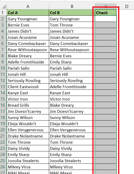
STEP 1: Create a new column.

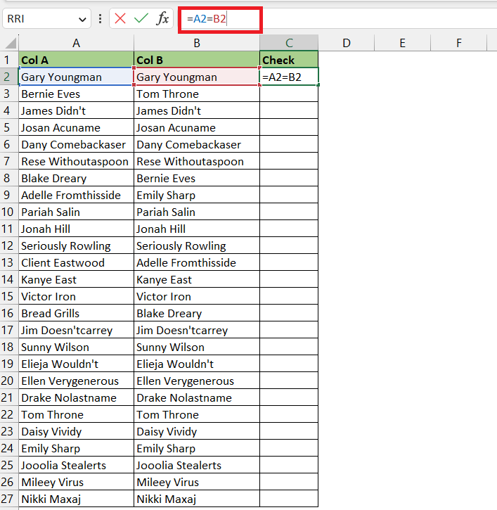
STEP 2: Input the two cells that you are trying to compare separated by an equal sign operator.

=A2=B2

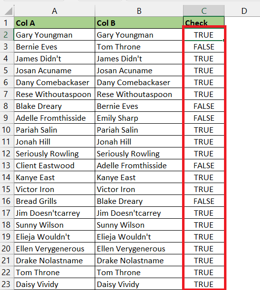
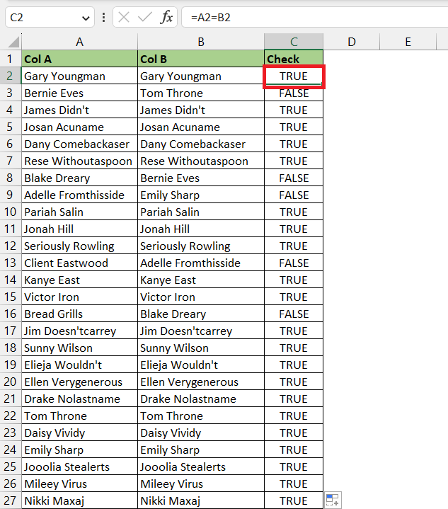
STEP 3: Copy the formula below to populate the formula for the remaining cells in the column.

You can see that the rows with matching values will return the value as TRUE otherwise it will return the value as FALSE.

 

Method 2: EXACT Function

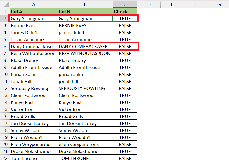
The Equal operator is used to compare cell values but it does not consider case sensitivity. The EXACT function is used specifically to compare text keeping in mind the distinction between uppercase and lowercase letters. It will return TRUE only if the values are identical in a case-sensitive manner as well.

Let’s compare two columns in this example using the EXACT function –

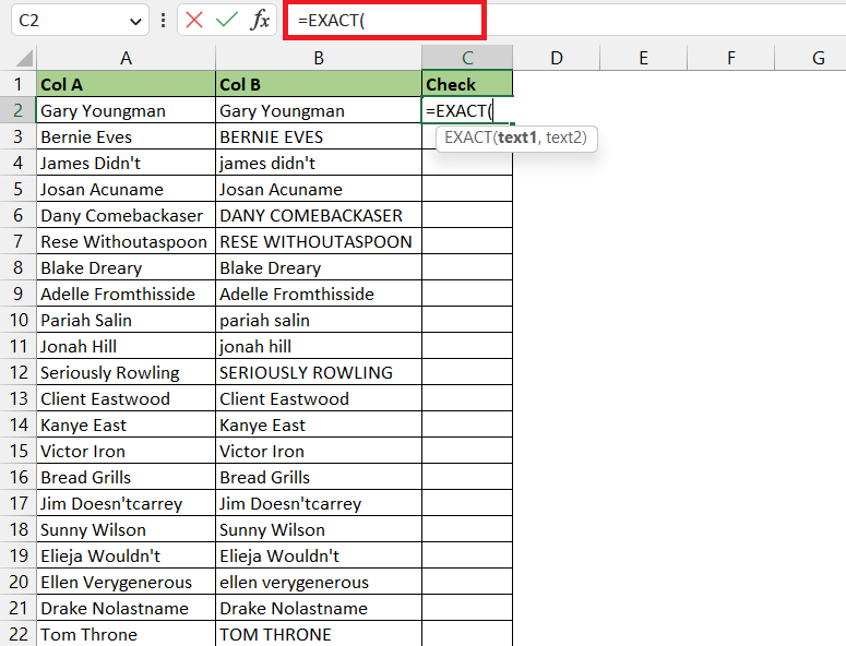
STEP 1: Enter the EXACT function.

=EXACT(

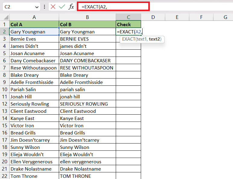
STEP 2: Enter the first argument i.e. the first text that you need to compare. Here, it is in cell A2.

=EXACT(A2,

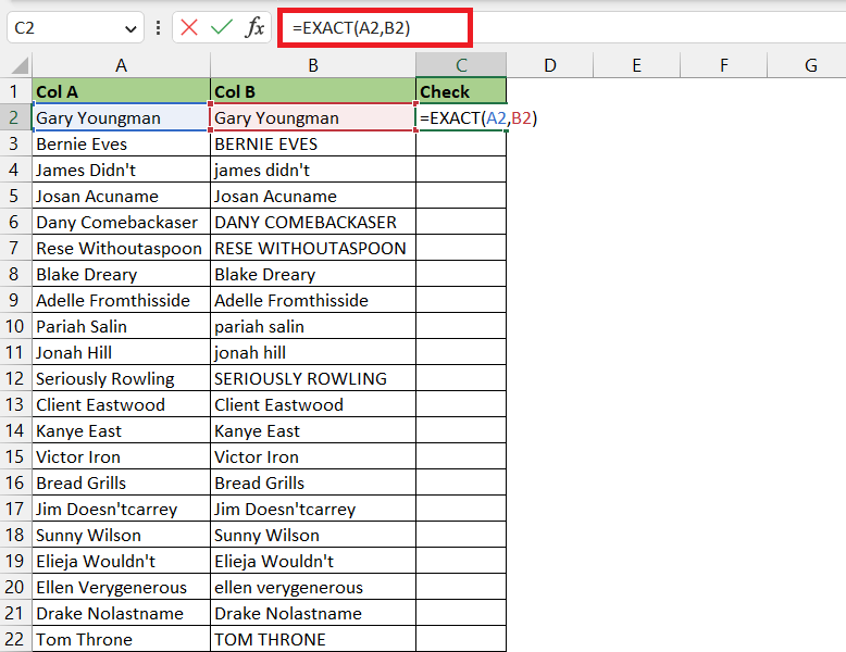
STEP 3: Enter the second argument i.e. the second text that you need to compare. Here, it is in cell B2.

=EXACT(A2,B2)

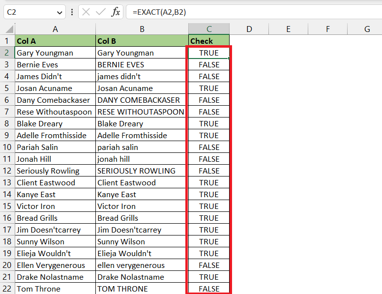
STEP 4: Copy the formula below to populate the formula for the remaining cells in the column.

You can see when the values in columns A and B are exactly the same in case sensitive manner, the function is returning the value as TRUE or else FALSE.

 

Method 3: IF Function

You can use the IF function in Excel to compare two columns and specify the desired output if the comparison is TRUE or FALSE. As compared to the equal operator, it helps you in providing more flexibility as opposed to an equal operator where you can only display boolean results – TRUE or FALSE.

Here’s an example –

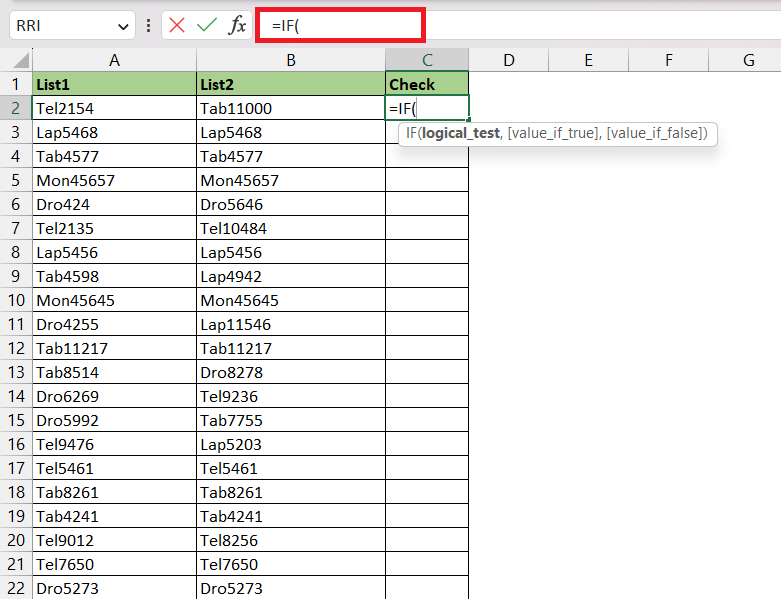
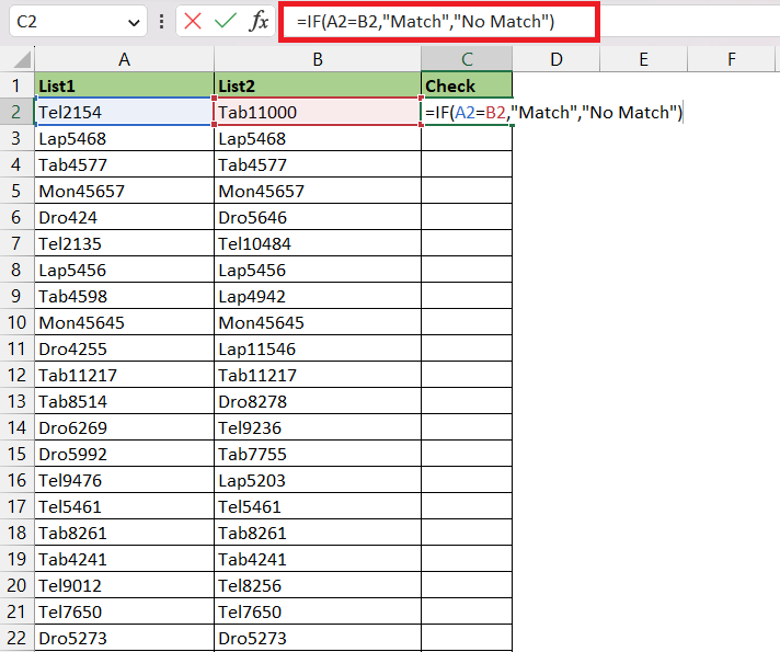
STEP 1: Enter the IF function.

=IF(

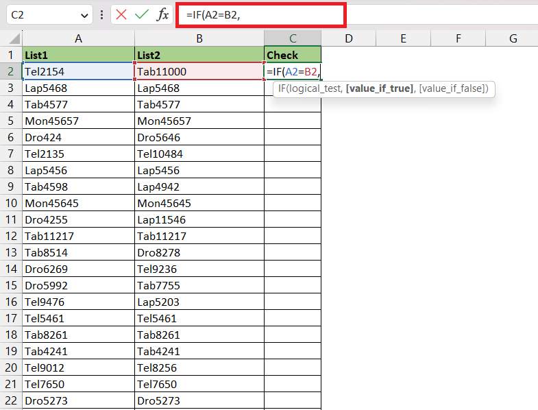
STEP 2: Enter the first argument i.e. the logical test.

=IF(A2=B2,

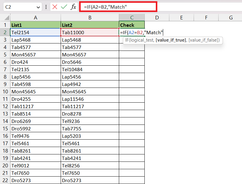
STEP 3: Enter the second argument i.e. the value if the condition is true.

=IF(A2=B2,”Match”,

STEP 4: Enter the third argument i.e. the value if the condition is false.

=IF(A2=B2,”Match”,”No Match”)

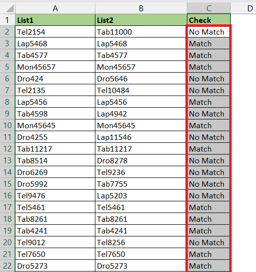
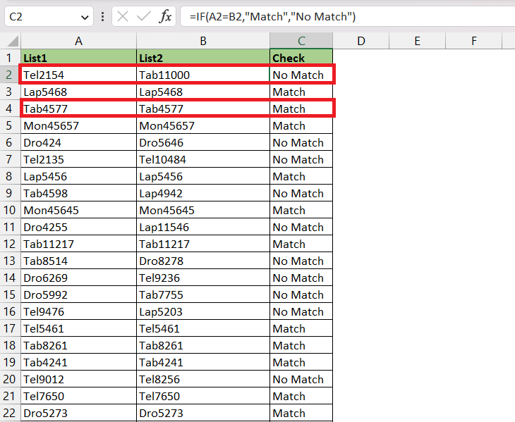
STEP 5: Copy the formula below to populate the formula for the remaining cells in the column.

You can see when the values in columns A and B are exactly the same, the function returns the value as TRUE or else FALSE.

 

Method 4: Conditional Formatting

To use conditional formatting to compare two columns in Excel, follow the steps below –

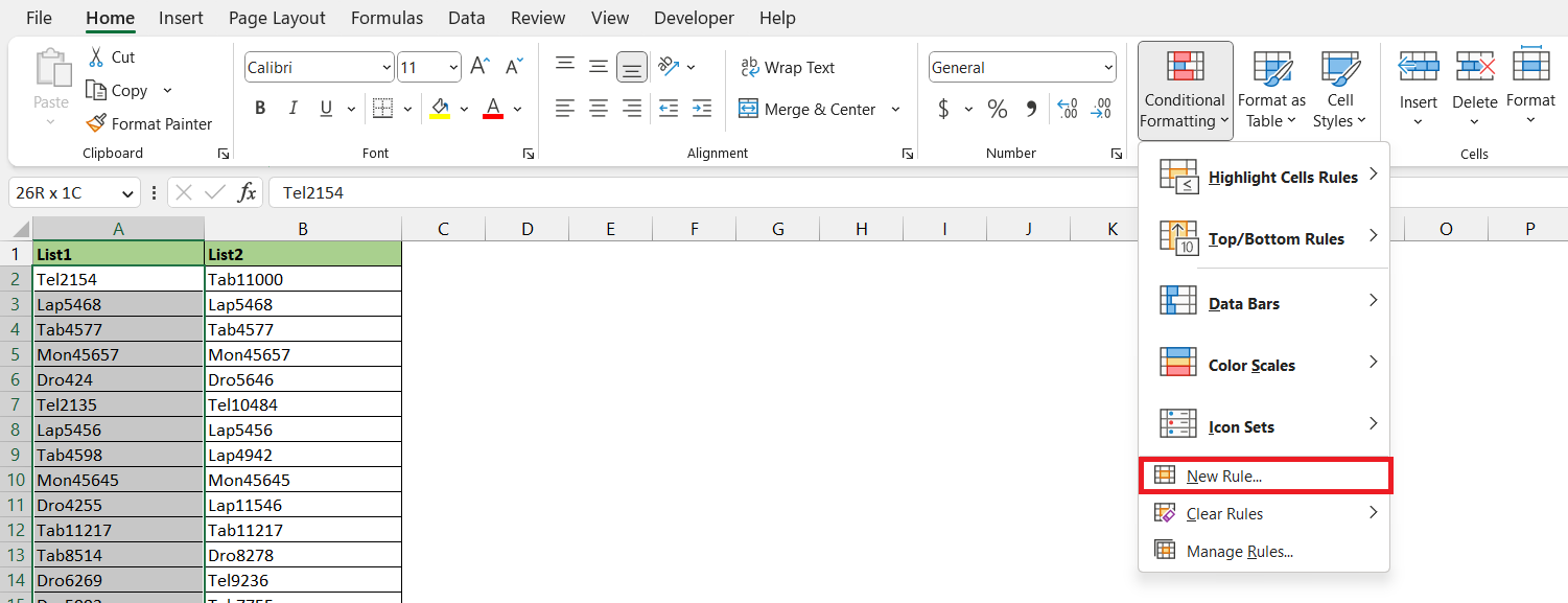
STEP 1: Select the cell range where you want the formatting to be shown.

STEP 2: Go to Home > Condition Formatting > New Rule.

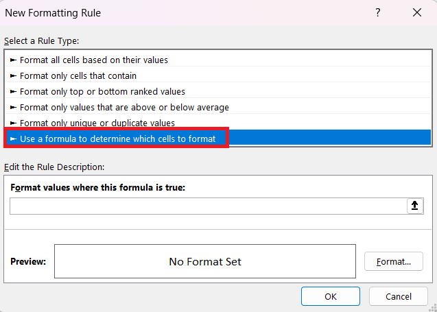
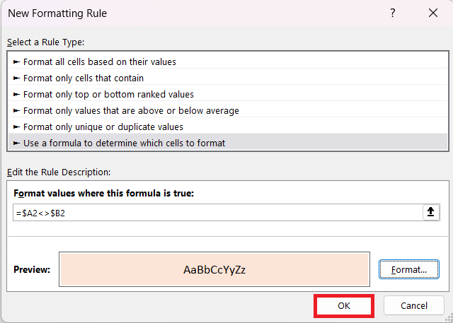
STEP 3: In the New Formatting Rule dialog box, select Use a Formula to determine which cells to format.

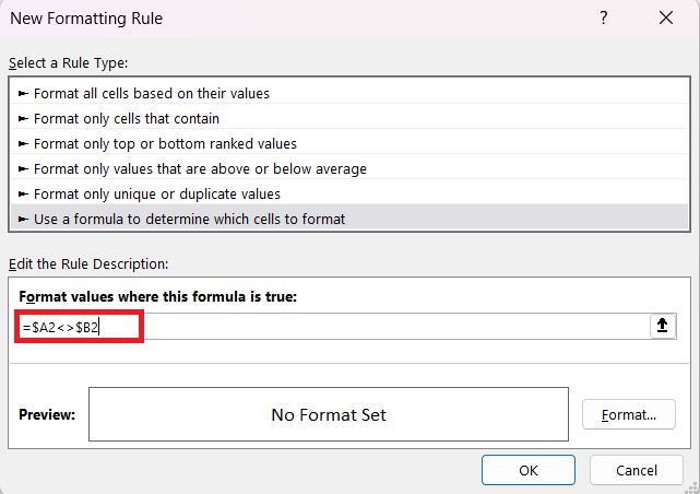
STEP 4: Type the formula stated below –

=$A2<>$B2

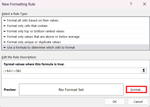
STEP 5: Click on the Format button.

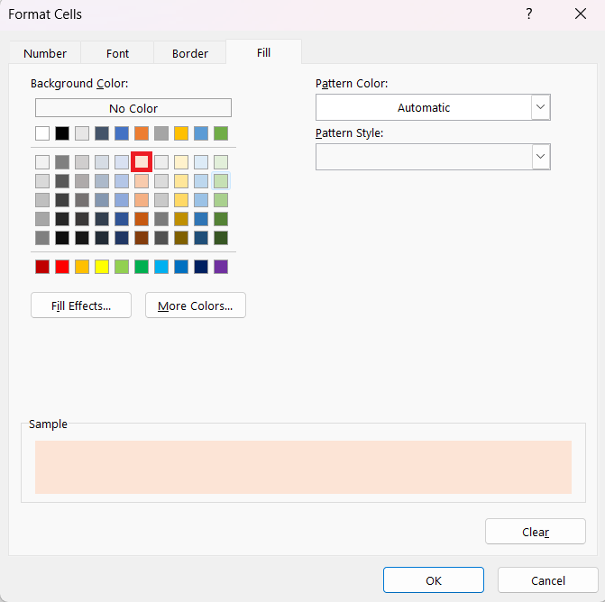
STEP 6: Under the Fill tab, select the light red color. Click OK.

STEP 7: Double-check the result under Preview and then click OK.

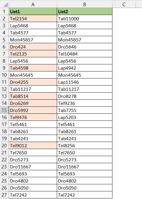
And Voila, you will see that the desired result has been achieved. The cell values in column A that do not match Column B will be highlighted in light red fill.

 

Method 5: MATCH Function

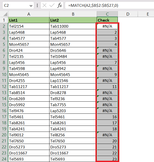
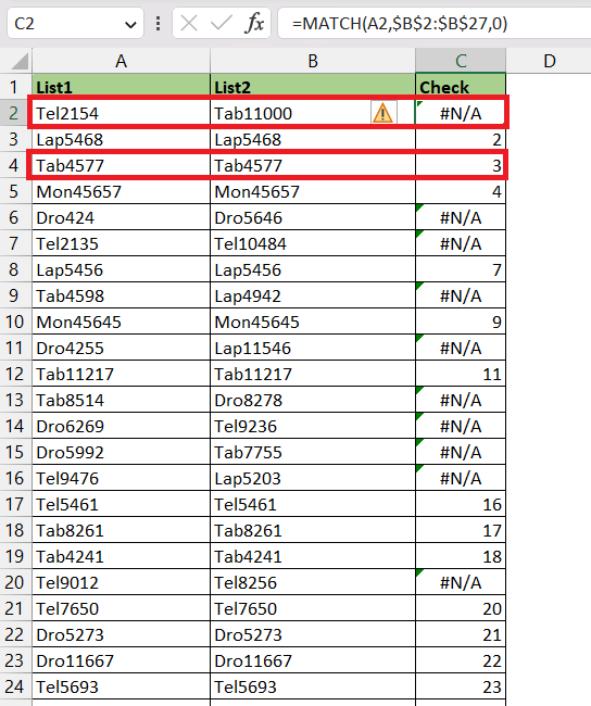
The MATCH function is typically used to return the position of an item in a range. But, you can also use it to compare two columns and check if a specific item in List1 exists in List2. The function will return the row position of that item in List2 hence confirming that it exists.  If you get a #N/A it means that the cell´s item does not exist in List2.

Let’s understand it better with an example –

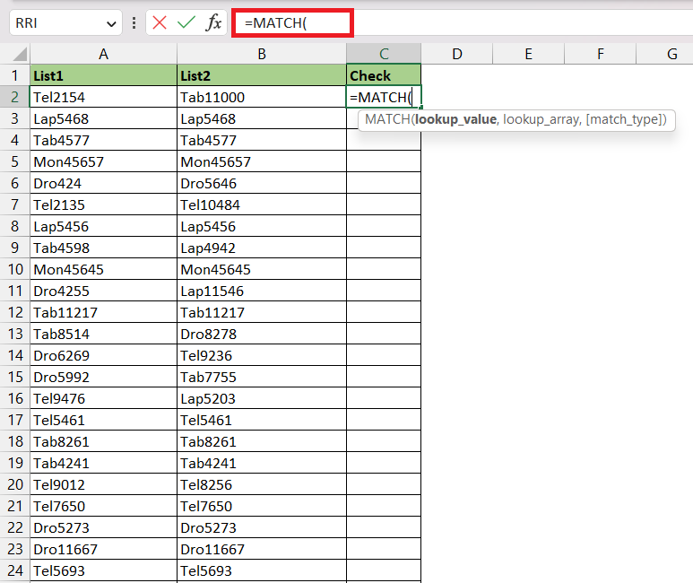
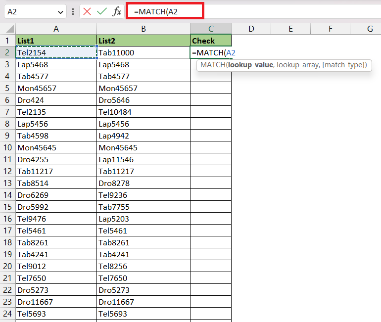
STEP 1: Enter the MATCH function.

=MATCH(

STEP 2: Enter the first argument – lookup_value. Here, it is mentioned in cell A2.

=MATCH(A2,

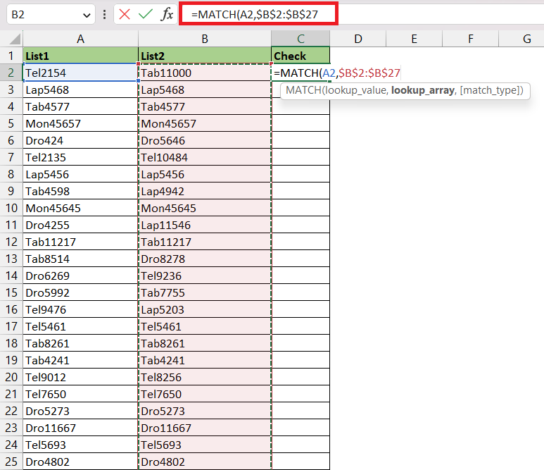
STEP 3: Enter the second argument – lookup_array. Here, it is the range B2:B30.

=MATCH(A2,$B$2:$B$27,

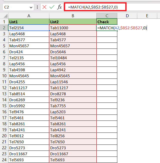
STEP 4: Enter the third argument – match_type. Here, it is 0 for an exact match.

=MATCH(A2,$B$2:$B$27,0)

STEP 5: Copy the formula below to populate the formula for the remaining cells in the column.

You can see when the values in columns A and B are the same, the function returns the value as a row number or else #N/A.

 

Method 6: Highlight Row Difference

You can easily highlight differences in value in each row using an in-built feature in Excel. It will provide you with an idea of how many lines in the columns differ in values.

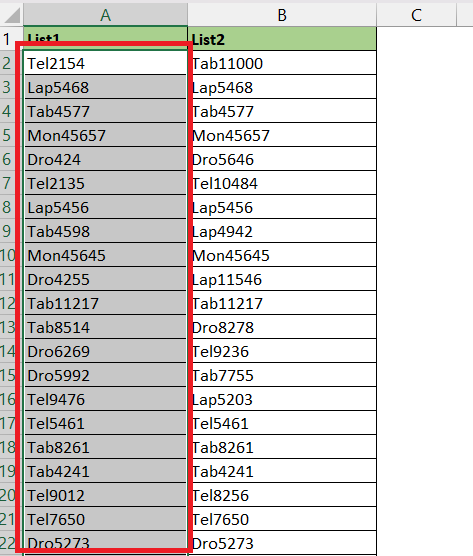
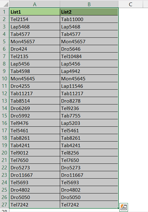
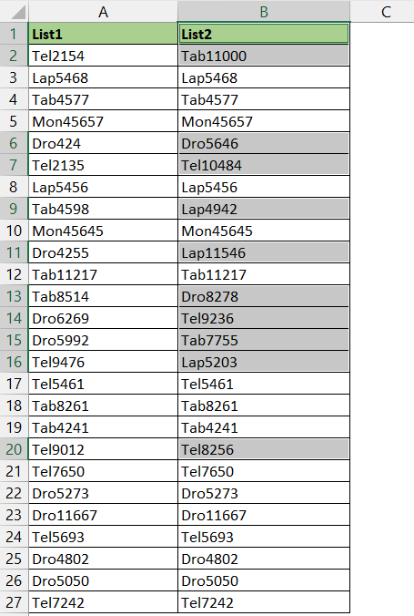
In the data below, you have two lists in Column A and Column B respectively.

Follow the steps below to compare two columsn and highlight row difference :

STEP 1: Select both columns.

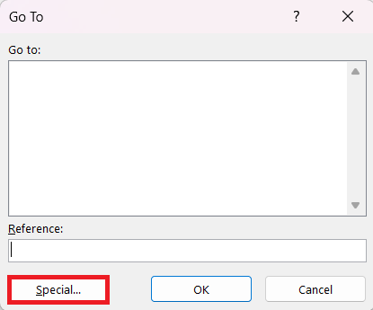
STEP 2: Go to Home > Find & Select > Go To Special or simply press keys Ctrl + G and Select Special to open the Go To Special dialog box.

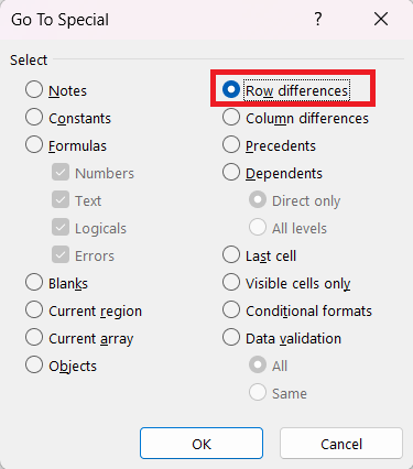
STEP 3: Select Row Difference and Click OK.

And, Voila!

All the values in List 2 that do not match the corresponding value in List 1 have been highlighted.

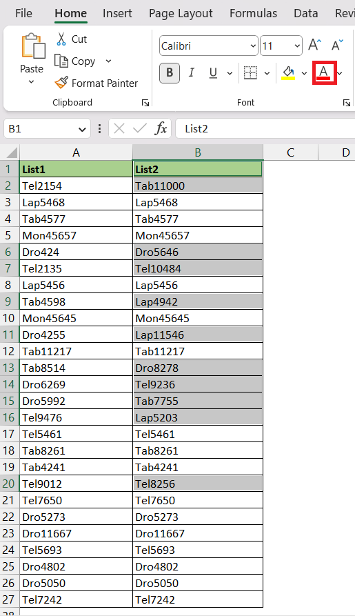
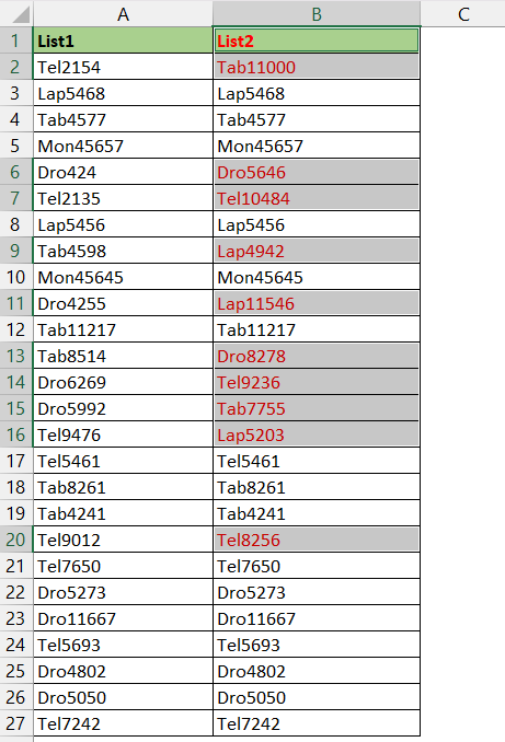
STEP 4: You can mark these cells with color as well. Go to Home > Font Color > Select Red.

This will permanently highlight the cells in red font color for future reference.