Conditional Format Based on Another Cell in Excel – Step by Step Guide

Conditional formatting in Microsoft Excel is a powerful tool that enhances the readability and analysis of data by automatically applying formatting based on cell values. This feature allows users to quickly identify trends, anomalies, and specific conditions in a spreadsheet. From simple color changes to complex formula-based rules, mastering conditional formatting can significantly improve data management and visualization.

Key Takeaways

• Understanding Basics: Conditional formatting applies styles like colors, icons, or data bars to cells based on their values, making data trends and outliers easily visible.
• Advanced Techniques: Beyond basic formatting, Excel offers advanced techniques, such as using formulas for dynamic conditions or visualizing data with color scales and icon sets.
• Custom Rules: Creating rules based on other cells’ values allows for dynamic and responsive formatting, essential for tracking and highlighting relevant data changes.
• Efficient Management: Organize and prioritize multiple formatting rules to ensure clarity and performance, using features like ‘Stop If True’ to prevent rule conflicts.
• Performance Optimization: For large datasets, keep formatting simple, apply it to necessary ranges only, and periodically review rules to maintain workbook efficiency and responsiveness.

 

Mastering Excel Conditional Formatting

Understanding the Basics of Conditional Formatting

Conditional formatting in Excel lets you automatically apply formatting—such as colors, icons, or data bars— to one or more cells based on the cell value. This can significantly enhance the readability and comprehension of a spreadsheet by allowing users to spot trends, anomalies, or specific conditions quickly.

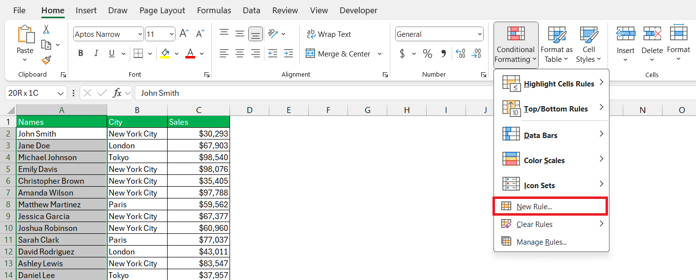
To get started, select your cells and navigate to the “Home” tab, where you’ll find the “Conditional Formatting” dropdown in the “Styles” group.

Here, you can choose from predefined formats like highlighting cells that contain certain values, or you can use the varied options to set your custom rules.

Exploring Advanced Conditional Formatting Techniques

When you’re ready to move beyond simple color changes and data bars, Excel’s conditional formatting offers a suite of advanced techniques to up your data game. You can use formulas to single out cells that meet complex criteria or even manipulate the format based on another cell’s value. Imagine color-coding a whole row based on a single cell’s status or setting up formats that change according to dynamic inputs or timeframes.

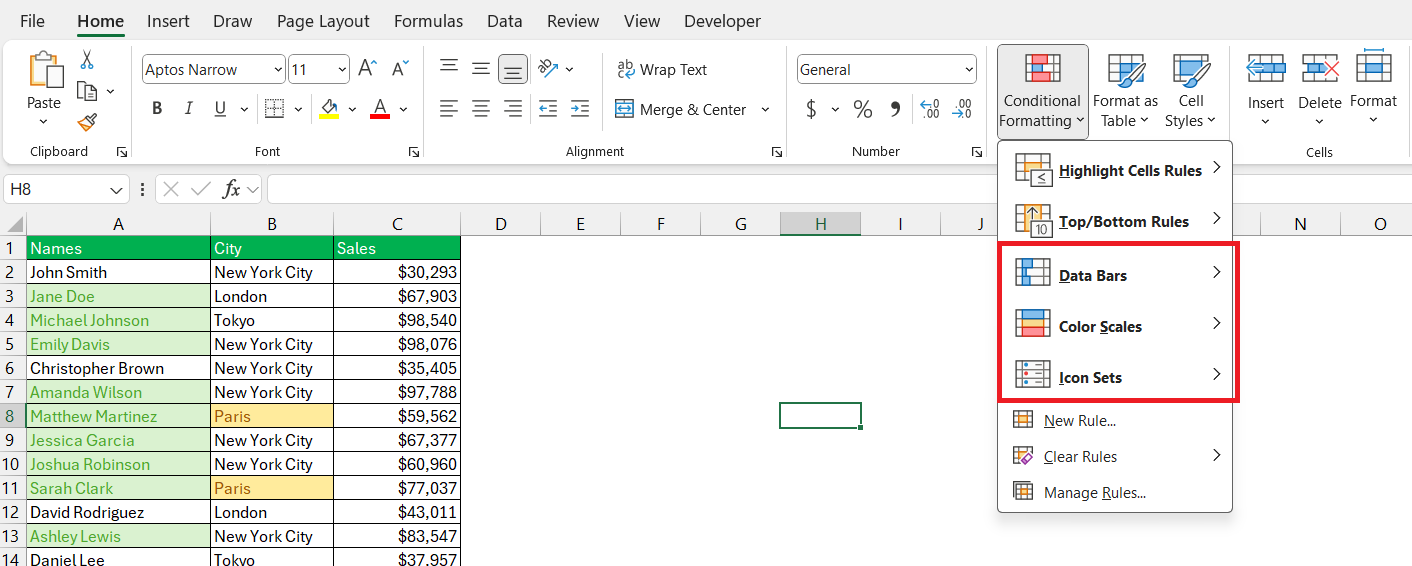
You can also tap into conditional formatting to create visualizations within your data. Color scales can shade cells across a spectrum to represent value ranges, while icon sets can append symbols to communicate information quickly, like using flags to signal priority tasks.

 

Crafting Custom Rules for Unique Scenarios

Setting Up Conditional Formats Based on Other Cells’ Values

Creating conditional formatting rules that reference the values of other cells allows for dynamic and responsive spreadsheets. This is particularly useful when you need to track changes across a dataset or highlight pertinent information relative to another field.

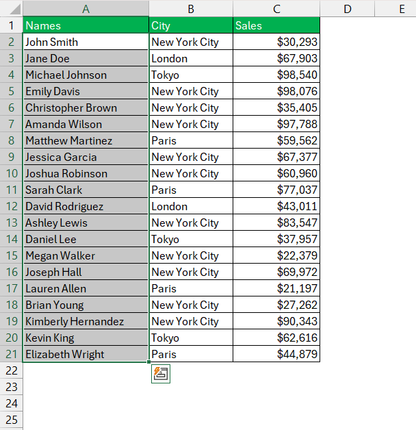
To set this up, you can use a formula to define the condition. For example, let’s say you want to highlight all the sales figures in a column that is greater than the target figure. By selecting your range and creating a new rule using a formula, you can reference the target sales.

Here’s a step-by-step approach:

STEP 1: Select the cells you want to conditionally format.

STEP 2: Go to “Conditional Formatting” and select “New Rule.”

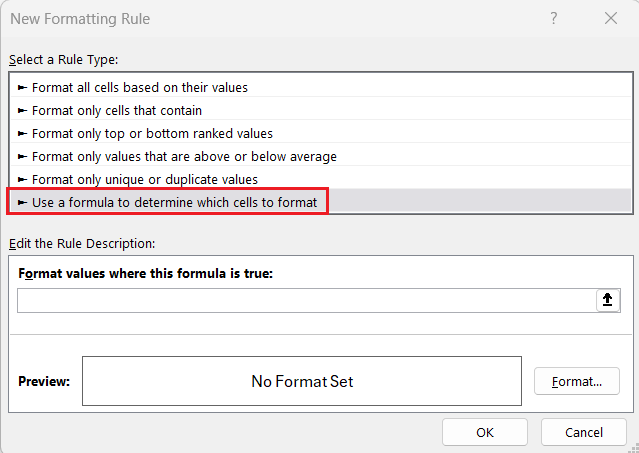
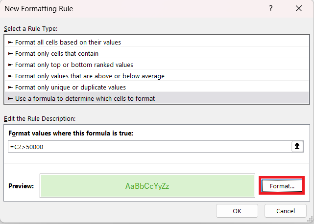
STEP 3: Choose “Use a formula to determine which cells to format.”

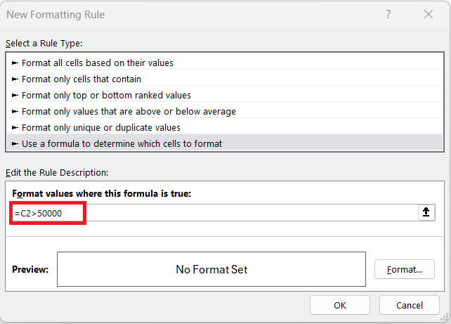
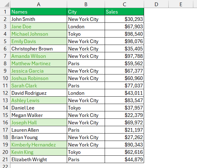
STEP 4: Enter the formula that references the other cell, such as =C2>50000 .

STEP 5: Set the desired format and click OK.

The selected format will be applied in column A based on the sales mentioned in column C.

Careful consideration of cell references ensures that your conditional formatting behaves as intended when your data changes.

Applying Complex Conditions with Formulas

Applying complex conditions with formulas in Excel’s conditional formatting can be game-changing. You can build rules that react to various scenarios, providing deeper insights and custom solutions for your data management tasks.

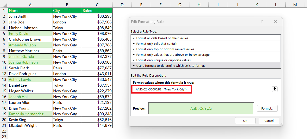
For example, using an AND or OR logical function lets you combine multiple conditions within a single rule. Imagine you want to highlight sales records where the sales exceed 50000 and the city is ‘New York City’. The formula in your conditional formatting rule could be =AND(C2>100, B2="New York City"), where column C has the sales amount, and column B indicates the city.

When crafting these sophisticated conditional formats, the actual writing of the formula is crucial. Conditional formatting is sensitive to the structure of the formula, making it essential to understand the precedence and compatibility of Excel functions and references.

 

Tips for Efficient Management of Formatting Rules

Organizing and Prioritizing Multiple Conditional Formats

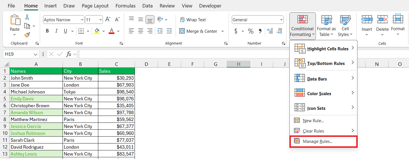
When you start to create multiple conditional formatting rules for a worksheet, organization and prioritization become crucial. Excel applies conditional formatting in the order of the rules listed in the “Manage Rules” dialog box, which means if two rules conflict, the first rule will take precedence.

To keep your conditional formats neat and functioning as intended, follow these steps:

• Regularly review your list of rules via the ‘Manage Rules’ window, accessible from the ‘Conditional Formatting’ dropdown menu.

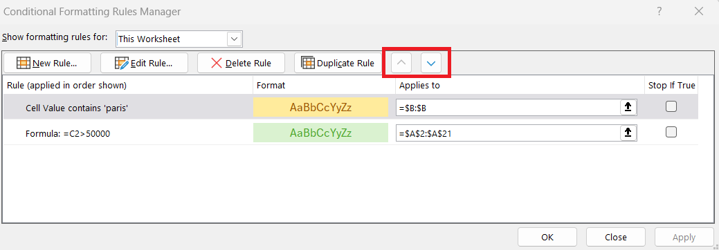
• Use the ‘Move Up’ and ‘Move Down’ buttons to arrange the rules in the order you want them to be applied. Conditions that are more specific or exceptions should generally be placed higher up the list than broader conditions.

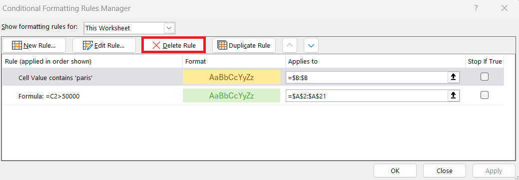
• If you find a rule is no longer necessary, don’t hesitate to delete it to simplify your formatting structure.

• Consider combining rules when possible. If two rules could be consolidated into one through a more cleverly crafted formula, it’s usually worth doing to minimize complexity.
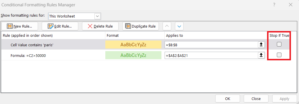
• Don’t forget to check the ‘Stop If True’ box when appropriate. If you have a rule whose criteria override subsequent rules, ticking this box will prevent other formats from being applied when the condition is met.

Maintaining an orderly list of conditional formats ensures that your worksheet remains readable and that the conditional formatting aids rather than hinders your data analysis.

 

Leveraging Conditional Formatting for Data Analysis

Identifying Trends and Patterns with Conditional Formatting

Conditional formatting is a remarkable tool for identifying trends and patterns within a dataset at a glance. With well-chosen formatting rules, you can visualize the flow of data over time, spot recurring events, and foreground anomalies that may require further investigation.

Here’s how this can be achieved:

• Data Bars: These fill the background of a cell with a length proportional to the cell’s value. When applied across a data series, they create a bar-chart effect within the cells, making it easier to see progression or regression over time.
• Color Scales: Using two or three shades, these scales provide an immediate heat-map effect. For instance, using a 3-color scale where red indicates lower values, yellow middle values, and green higher values can quickly show you where the peaks and valleys are in your data.
• Icon Sets: Choose icons that vary not just in color but in shape to denote up and down trends, stability, or outliers.

It’s beneficial to use these tools thoughtfully. For example, in tracking monthly sales data, applying a gradient color scale will allow you to see which months had the highest sales and which ones may have seen a dip, possibly indicating a seasonality you could capitalize on or work to improve.

By smartly applying conditional formatting, you enable users to decode trends and patterns without the need for in-depth analysis or reading through rows of figures, making data accessible to a wider audience.

 

Optimizing Conditional Formatting for Performance

Best Practices for Large Datasets

When you’re working with large datasets, using conditional formatting efficiently is key to ensure your spreadsheet remains responsive and your insights are clear. Here are some best practices to keep in mind:

1. Keep It Simple: With numerous rows and columns of data, it’s best to minimize the number of conditional formatting rules you apply. Too many rules can slow down performance and confuse rather than clarify.
2. Use Formulas Sparingly: When writing formulas for conditional formatting, keep them as straightforward as possible. Complex formulas can be resource-intensive, especially when applied to a vast range.
3. Apply Formatting to Minimum Necessary Range: Rather than blanket-formatting entire columns or rows, focus on exactly the range where data is present. This prevents Excel from processing unnecessary cells, enhancing performance.
4. Use Cell Styles: Define cell styles for frequently used formats. This allows for better consistency and easier adjustments across large ranges.
5. Periodic Review: Regularly review your formatting rules to ensure that they are all serving a purpose. Remove any that are outdated or redundant to maintain cleanliness and efficiency.

Adhering to these practices will help maintain the speed and functionality of your workbook, while still allowing you to visually analyze large datasets effectively.

Remember, the overarching goal of conditional formatting, even with large datasets, is to highlight significant data points and trends without overwhelming users with too much visual information.

Conditional Formatting and Workbook Size Considerations

While conditional formatting is a powerful tool for data visualization, it can have implications for your workbook’s size and performance—particularly when you’re dealing with extensive datasets. Every rule you add increases the complexity of the workbook, which can lead to increased file sizes and longer processing times.

Here are some considerations to minimize the impact:

1. Use Formats Efficiently: Limit the use of different font styles, borders, and colors. The more unique styles you have, the more information Excel has to store.
2. Avoid Volatile Functions: Some functions, like TODAY() or INDIRECT(), trigger recalculations more often. When used in conditional formatting, these can slow down your workbook.
3. Focus on Relevant Data: Apply conditional formatting only to cells that will benefit from it. For instance, instead of formatting entire columns, limit the range to the cells that actually contain data.
4. Streamline Rules: If multiple rules can be combined into a single, more inclusive rule with the same format, do so.
5. Clean Up Regularly: Audit your conditional formatting rules and remove any that are unnecessary or redundant. This can reduce file size and improve performance.

Considering these factors will help maintain your Excel workbook’s efficiency and ensure that conditional formatting remains a helpful and not a hindering tool.

Always strive to strike a balance between a visually informative worksheet and one that maintains optimal performance.

 

FAQ: Honing Your Conditional Formatting Mastery

What is Conditional Formatting in Excel?

Conditional formatting in Excel is a feature that allows you to apply specific formatting to cells that meet certain criteria. It’s a fantastic way to visually highlight important information, identify trends and exceptions, and make data analysis more intuitive. With conditional formatting, you can change the color of cells, apply data bars, color scales, and icon sets automatically based on cell values.

How Do I Apply Conditional Formatting to an Entire Row Based on One Cell’s Value?

To apply conditional formatting to an entire row based on one cell’s value, you must use a formula rule. First, select the rows or tables. Then, go to the ‘Conditional Formatting’ option, choose ‘New Rule,’ and select ‘Use a formula to determine which cells to format.’ Enter a formula that references the cell in question. For example, if column A holds the value to check against, your formula could be =$A1="Specific Value". Set the format you want, and apply the rule.

Can I Use Conditional Formatting to Compare Values Across Different Worksheets?

Yes, you can use conditional format to compare values across different worksheets in Excel. To do this, you’ll need to write a formula in the conditional formatting rule that references the cell in the other worksheet. When writing this formula, use the full reference, including the worksheet name. For example, if you’re comparing a cell in Sheet1 to a value in Sheet2, your formula might look like =Sheet1!A1 > Sheet2!A1. Apply this formula as the basis for your formatting rule.

What Are Some Ways to Avoid Common Mistakes When Using Conditional Formatting?

To avoid common mistakes in conditional formatting, start by carefully planning your rules. Keep these tips in mind:

• Verify that cell references are correct—use absolute references where necessary.
• Always start your formula with the top-left cell in the selected range.
• Ensure rules don’t overlap unless intended, using the ‘Stop If True’ checkbox.
• Regularly manage and review your rules to keep them organized.
• Avoid excessive conditional formatting in large datasets to prevent slow performance.

By following these guidelines, you can maintain an efficient and error-free conditional formatting setup.

Is There a Limit to the Number of Conditional Formatting Rules I Can Set?

Excel does impose a limit on the number of conditional formatting rules you can set for a given dataset, which is typically generous but depends on the version of Excel you’re using and the complexity of your rules. For instance, older versions of Excel may have lower limits compared to the latest versions. However, it’s worth noting that while you might not hit an absolute limit, overextending with too many rules can slow down your workbook. It’s best to use conditional formats judiciously and consolidate rules when possible for optimal performance.