How to Compare Two Lists in Excel Fast!

Comparing lists in Microsoft Excel is a vital skill for ensuring data accuracy and integrity, whether for personal use or professional projects. This process involves identifying matches and discrepancies between datasets, which is crucial for tasks like financial reconciliation, inventory management, and data synchronization. By leveraging Excel’s powerful tools, such as conditional formatting and advanced formulas, users can streamline the comparison process and make informed decisions based on precise data analysis.

Key Takeaways:

• Simple Comparisons with the Equal Sign Operator: Use =A2=B2 to quickly identify matches (TRUE) and discrepancies (FALSE) in small datasets.
• Visual Comparisons with Conditional Formatting: Apply conditional formatting to color-code matches and differences, making error-spotting immediate and visual.
• Advanced Analysis with IF Conditions: Implement =IF(A2=B2, “Match”, “Difference”) for clear, customized feedback on data comparisons, enhancing data integrity.
• Deep Comparisons with Excel Formulas: Leverage VLOOKUP, MATCH, and INDEX for complex data comparisons, turning raw data into actionable insights.
• Efficient Filtering Techniques: Use Excel’s filtering features to dynamically extract and review matching or differing data, ideal for ongoing data review tasks.

 

Introduction to List Comparison in Excel

Why Comparing Lists is Essential

List comparison in Microsoft Excel is an essential skill for both personal and professional users. Whether one is reconciling finances, syncing contact lists, or analyzing inventory data, comparing lists helps ensure accuracy and completeness.

It flags discrepancies and serves as a foundational step for data verification, enabling a thorough analysis and informed decision-making. In the dynamic world of data, keeping content precise and error-free is crucial, and list comparison serves as an indispensable tool for achieving that precision.

Overview of Techniques for List Comparison

Comparing lists in Excel can be tackled using various techniques, each suited to different scenarios and complexity levels. Whether working with rows of sales figures or columns of inventory items, one can harness the equal sign operator for simple side-by-side comparisons, or delve into conditional formatting for a visual display of matches and differences.

For more intricate analysis, formulas like IF, VLOOKUP, or MATCH come into play, allowing for dynamic data examination. From basic visual cues to advanced array formulas, the range of methods means one will always find an approach that fits the task at hand, transitioning list comparison from a potential chore to a powerful, streamlined process.

 

Getting Started with Basic Comparisons

The Straightforward Equal Sign Operator Method

One of the simplest methods to compare two Excel columns is using the Straightforward Equal Sign Operator. To employ this, one creates a new column where each cell contains a formula comparing the corresponding cells in the two lists.

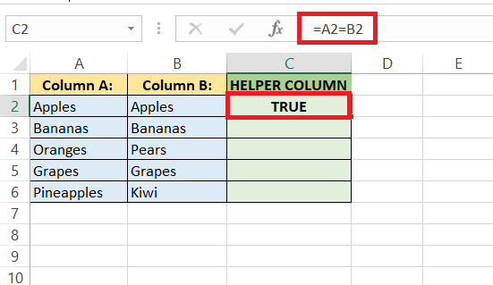
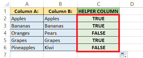
It looks something like =A2=B2, and it churns out TRUE if the cells match and FALSE if they don’t. This method is great for quick checks on exact matches and offers an immediate visual reference for data consistency. It’s particularly useful when handling smaller datasets where a rapid, line-by-line verification is all that’s needed.

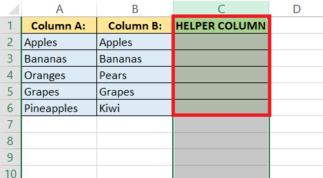
STEP 1: Insert a new column next to the lists.

STEP 2: In the first cell of the new column, enter the formula: =A2=B2.

STEP 3: Drag the fill handle down to copy the formula to all cells in the new column. Excel will display TRUE if the cells match and FALSE if they don’t

Using Conditional Formatting for Visual Comparisons

Conditional Formatting is a fantastic feature in Excel that can make visual comparisons of lists much more straightforward. By selecting the range of data one wishes to compare and to navigate to the ‘Home’ tab to choose ‘Conditional Formatting’, users can set rules to highlight cells with duplicate or unique values. This allows one to quickly spot similarities or differences by color-coding the cells.

For instance, one might choose a green fill for matches and red for discrepancies, thereby making the patterns in the data pop out instantly. It’s an efficient way to process data visually, reducing the time spent on spotting errors or inconsistencies.

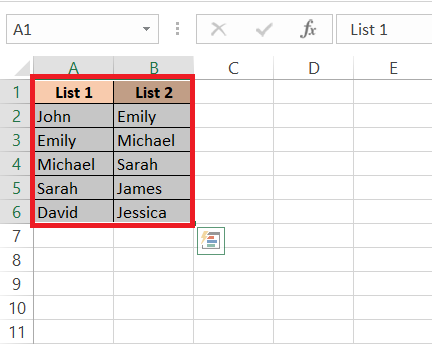
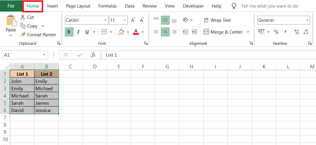
STEP 1: Select both lists.

STEP 2: Go to the ‘Home’ tab.

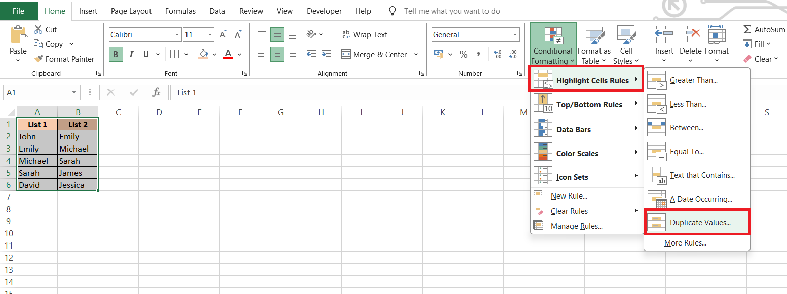
STEP 3: Click on ‘Conditional Formatting’. Choose a rule like ‘Highlight Cells Rules’ > ‘Duplicate Values’.

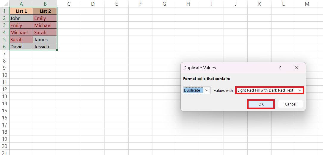
STEP 4: Customize the setting based on the color you want and Click ‘OK’.

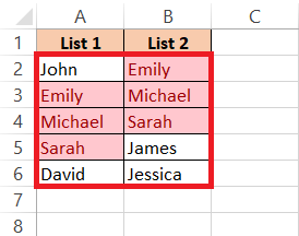
RESULT:

 

Advanced Methods for Professional Analysis

Utilizing IF Conditions to Highlight Differences

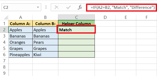
Going beyond basic comparison with the IF function opens up a world of possibilities in Excel. By using the IF condition to compare two columns, one can output a custom message based on their criteria. A simple formula like =IF(A2=B2, "Match", "Difference") can tell at a glance whether the entries in two cells are the same.

This method provides clear and customized feedback on the data, making it incredibly useful for detecting variances and maintaining data integrity. It’s particularly handy for reporting purposes where one might need to categorize data based on match status, and for more complicated comparisons that require specific actions based on the outcome.

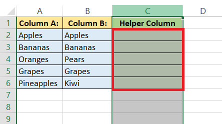
STEP 1: Insert a new column next to the lists.

STEP 2: In the first cell of the new column, enter the formula: =IF(A2=B2, “Match”, “Difference”).

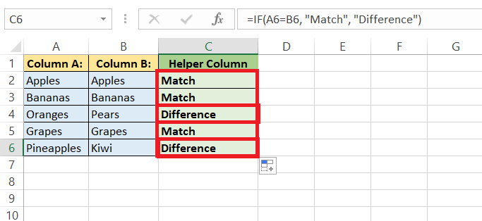
STEP 3: Drag the fill handle down to copy the formula to all cells in the new column. Excel will display “Match” if the cells match and “Difference” if they don’t.

Exploring the Power of Excel Formulas for Deep Comparisons

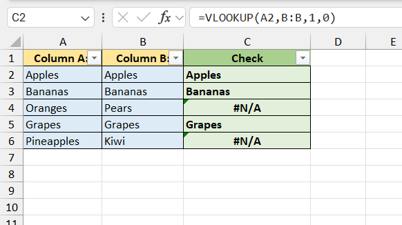
Excel formulas offer an immense degree of flexibility for deep data comparisons, enabling one to take their analysis to the next level. Functions like VLOOKUP, MATCH, and INDEX can be configured to find not just direct matches, but also similarities and relationships within and across datasets.

With these tools, one can perform lookups that factor in a wide array of conditions, retrieve additional data based on comparison results, or even pinpoint discrepancies across multiple criteria. Deep comparisons with Excel formulas can transform raw data into meaningful insights and support both fine-grained analysis and big-picture strategies.

 

Efficiently Identifying Matches and Differences

The Row Difference Technique Made Simple

The Row Difference technique in Excel is an elegant way to catch discrepancies in data that’s arranged row-wise. Even if you haven’t employed it previously, understanding this tool is quite straightforward:

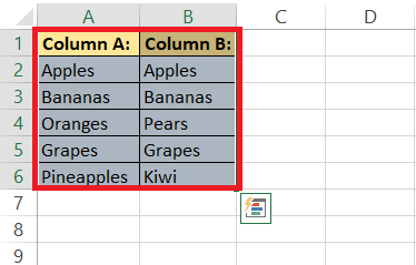
STEP 1: Begin by selecting the data one wishes to compare.

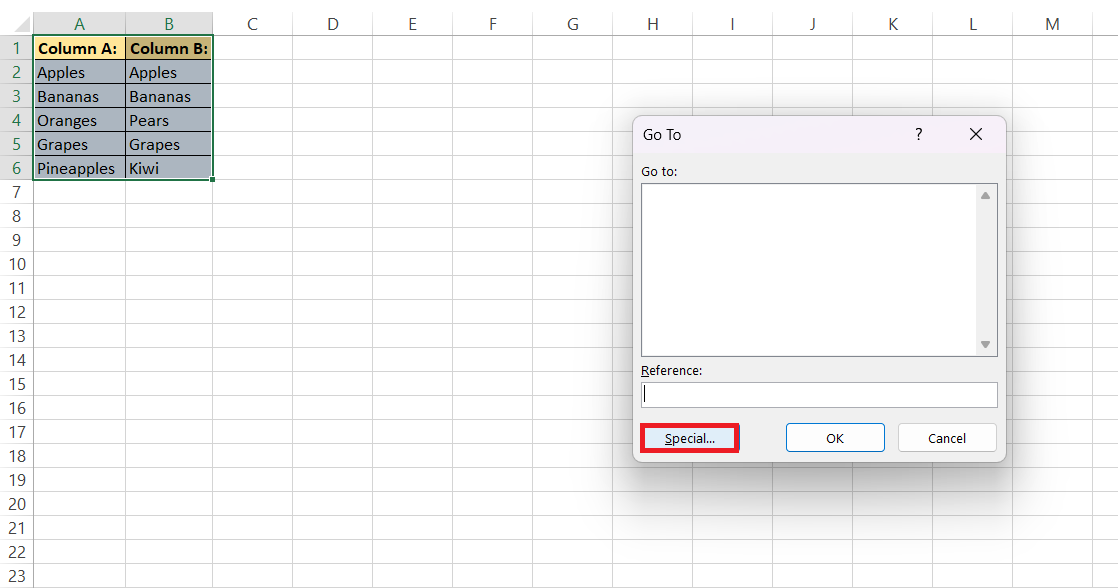
STEP 2: Then invoke the “Go To Special” tool by pressing the “F5” key and selecting “Special.”

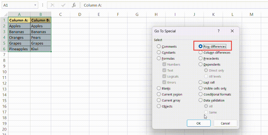
STEP 3: Within this menu, choose the “Row differences” option and click “OK.

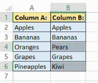
Now you have your row differences!

Excel now highlights cells that deviate from the comparison row, enabling one to easily spot the differences. One can further enhance the visibility by filling these cells with color. This technique excels when analyzing data where one expects consistency across rows, such as repeated entries in ledger books or similar segments of inventories.

Harnessing Filters to Extract Matching Data

Filters in Excel are particularly handy when you’re looking to sift through sizeable lists to extract and examine matching data efficiently. With just a few clicks, you can set up filters to either include or exclude specific types of information.

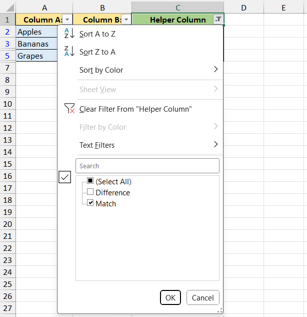
Let’s say you’ve used a formula to identify which cells in two columns match or not; applying a filter can then quickly show you all instances that meet your chosen criteria—like “Match” or “Difference”.

What’s great is that these filters are dynamic, which means as your data changes or grows, just reapply the filter to update your view. This method is phenomenal for recurring data review tasks where you want to regularly track new matches or differences as data evolves.

 

FAQs: Mastering List Comparison in Minutes

How can I compare two lists in Excel quickly?

To quickly compare two lists in Excel, use the Conditional Formatting feature to highlight differences. Select your list range, go to the ‘Home’ tab, click ‘Conditional Formatting’, then ‘Highlight Cell Rules’, and choose ‘Duplicate Values’. Adjust the formatting options to differentiate between matches and differences visually.

What is the best way to highlight differences between two columns in Excel?

The best way to highlight differences between two columns in Excel is by using Conditional Formatting with a custom formula. Select your data, then go to ‘Conditional Formatting’ under the ‘Home’ tab. Choose ‘New Rule’, ‘Use a formula’, and enter =A1<>B1. Set a format for highlighting and apply it to see the differences.

How do I compare two lists in Excel to find differences?

To find differences between two lists in Excel, you can use the formula =IF(ISERROR(MATCH(A1,B:B,0)),"No Match","Match") in a new column next to your first list. This will display “No Match” for items in List A not found in List B. Copy the formula down the column to check each item.

How do you compare two lists and return unique values in Excel?

To compare two lists and return unique values in Excel, you can use a combination of the IF and COUNTIF functions. Enter the formula =IF(COUNTIF(B:B, A1)=0, A1, "") into a new column beside your first list to output unique values from List A that aren’t in List B. Drag to fill the formula down.

Why is it useful to compare two columns in Excel?

Comparing two columns in Excel is useful for pinpointing discrepancies, synchronizing data, and ensuring consistency across records. It’s invaluable for tasks like reconciling accounts, updating databases, and validating entries, making it a cornerstone for data integrity and informed decision-making in diverse applications.