The VLOOKUP function in Microsoft Excel is a powerful tool designed to search for specific pieces of information within a dataset and retrieve corresponding data from another column. It simplifies the process of data retrieval by automating searches and extraction.
Key Takeaways
- The VLOOKUP function is essential for those claiming proficiency in Excel and is often a determinant of expertise in job interviews.
- Mastery of VLOOKUP is a significant skill, as highlighted by its frequent use in day-to-day Excel tasks.
- The tutorial provides a comprehensive guide, including syntax and practical examples, to help users thoroughly understand VLOOKUP.
Download the workbook and follow along with the tutorial on How to use VLOOKUP in Excel – Download excel workbookVLOOKUP-in-Excel.xlsx
Embracing the Versatility of VLOOKUP
VLOOKUP Function is a cornerstone function in Excel widely celebrated for its ability to streamline data analysis. Excel users embrace VLOOKUP because of how it simplifies the process of searching for specific information across large and complex datasets. It’s a versatile tool that reduces the necessity for manual searches, making it a favorite among financial analysts, marketers, and anyone who deals with data regularly.
The Significance of Lookup Values in Data Analysis
Lookup values are the heartbeat of data analysis in Excel. They are the unique identifiers that allow users to search for related information in a dataset. Whether it is text, numbers, or URLs, as long as the lookup value in your formula matches the corresponding value in your dataset, VLOOKUP in Excel can seamlessly retrieve the associated data you need. This becomes immensely valuable when dealing with extensive databases where pinpointing related entries manually would be like finding a needle in a haystack. By utilizing lookup values effectively, data analysts can ensure accuracy, save time, and enhance productivity in their workflows.
Table of Contents
Getting Started with VLOOKUP
Understanding VLOOKUP’s Syntax and Parameters
To harness the power of VLOOKUP in Excel, it’s crucial to understand its syntax and the function of its parameters. The syntax for a basic VLOOKUP formula in Microsoft Excel is as follows:
Let’s break down each component:
lookup_value: This is the value you want to search for in the first column of your table. This can be a number, text string, or a cell reference that houses the value you’re looking for.table_array: This is the range of cells that contains the data you want to retrieve. The first column in this range should contain the lookup values.col_index_num: This number represents the column in the table_array from which to retrieve the matching value, with the first column being number 1.[range_lookup](optional): This argument determines whether you want to find an exact match (FALSE) or an approximate match (TRUE or omitted). For exact matches, use FALSE. To look approximate match, the first column of your table must be sorted in ascending order, and you can use TRUE or simply omit this argument.
Understanding these parameters is the key to constructing effective VLOOKUP formulas and making your data work for you.
Setting Up Your First VLOOKUP Formula
Getting started with your first VLOOKUP in Excel is easier than you might think. Follow these step-by-step instructions to set up a basic VLOOKUP example:
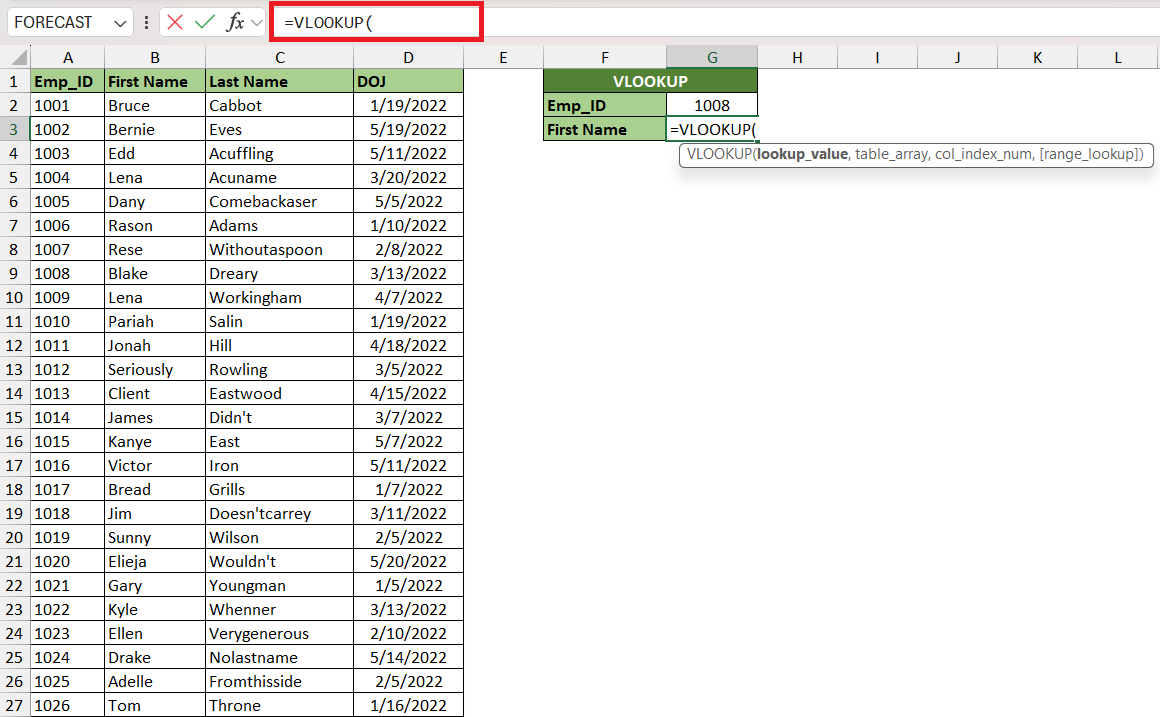
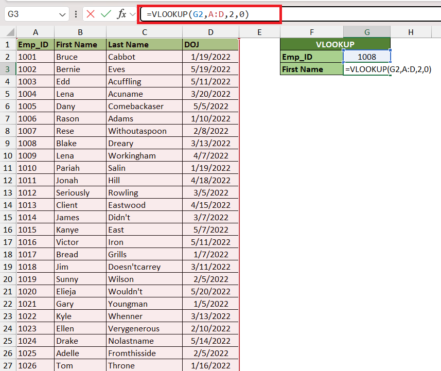
STEP 1: Enter =VLOOKUP() into the formula bar or use the Formula Builder for assistance.
=VLOOKUP
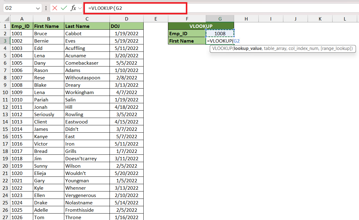
STEP 2: Fill in the ‘lookup_value.’ This can be a specific value or a cell reference.
=VLOOKUP(G2
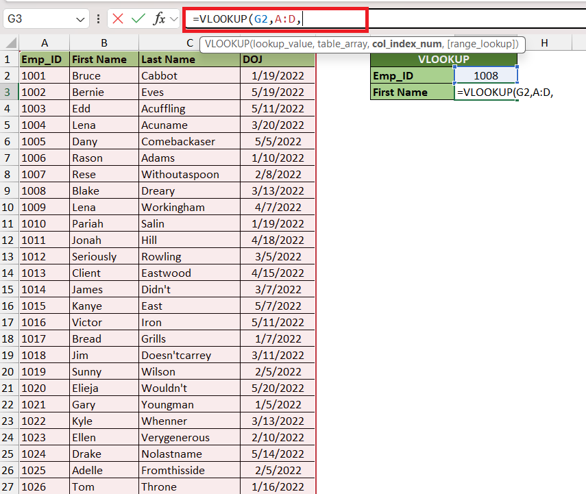
STEP 3: Define the ‘table_array’ by selecting the range of cells that contains the data you want to retrieve.
=VLOOKUP(G2,A:D
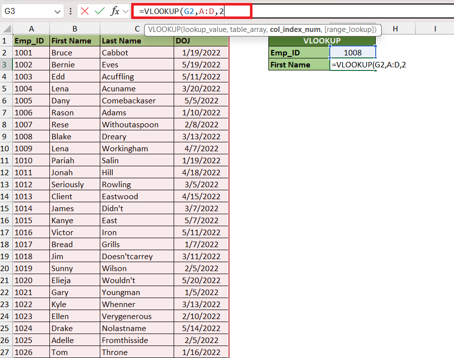
STEP 4: Enter the ‘col_index_num’ that corresponds to the column number in the ‘table_array’ from which to pull the data.
=VLOOKUP(G2,A:D,2
STEP 5: Choose your ‘range_lookup’ preference by entering TRUE for an approximate match or FALSE for an exact match.
=VLOOKUP(G2,A:D,2,0)
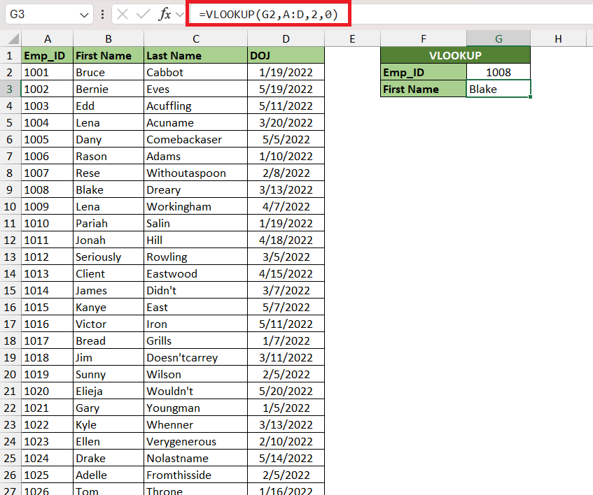
STEP 6: After filling in the formula parameters, press ‘Enter’ to execute the formula.
Check to see if the returned result matches your expectations. If it doesn’t, double-check your formula parameters for any errors.
Remember, your first attempt at a VLOOKUP formula could involve some trial and error. However, as you become familiar with the function’s structure and capabilities, it will become an indispensable part of your Excel toolkit.
Diving Deeper Into VLOOKUP Functionality
Handling Exact and Approximate Matches Effectively
When working with VLOOKUP in Excel, one crucial decision you’ll make is whether to search for an exact or approximate match. Understanding how to handle these two options effectively will significantly enhance the accuracy of your data retrieval.
Exact Match:
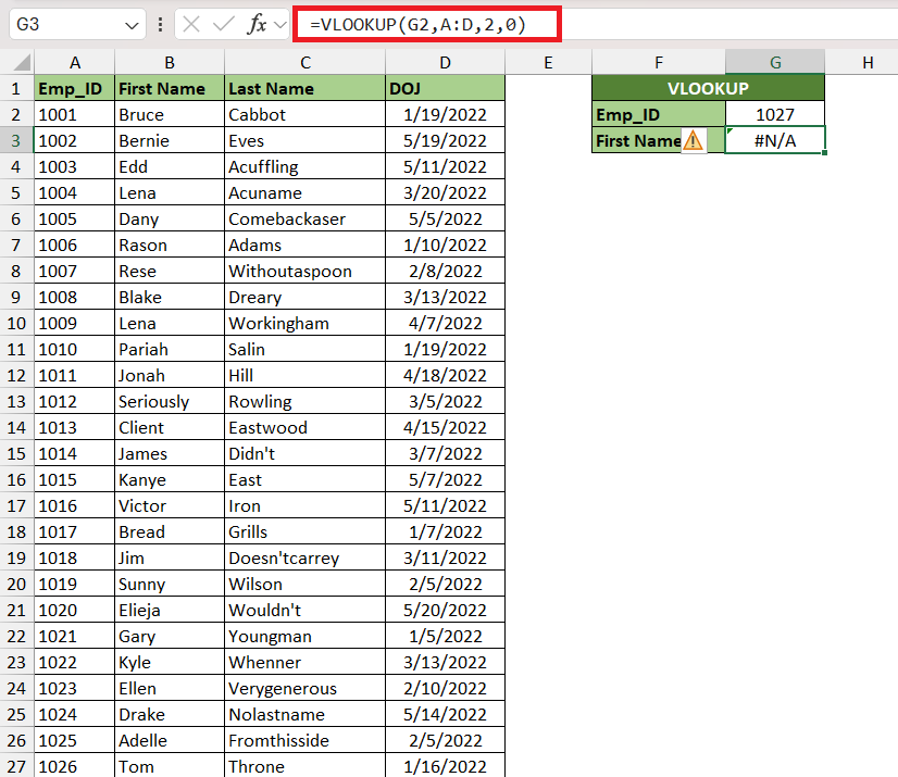
For an exact match, the final parameter of the VLOOKUP function should be set to “FALSE” OR “0”. In this mode, VLOOKUP will search for a value that corresponds exactly to your ‘lookup_value’. If there is no exact match, Excel will return an #N/A error, indicating that the exact value cannot be found in the first column of your ‘table_array’.
Example:
Result: #N/A
Approximate Match:
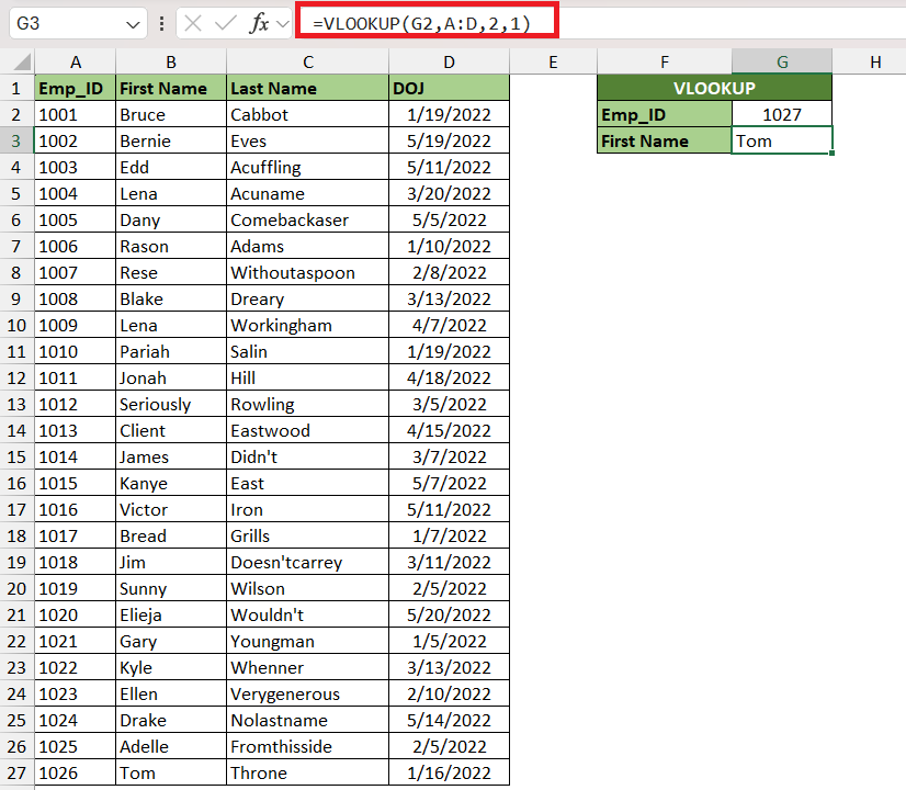
On the other hand, if your needs are more flexible or if an exact match might not always be present, you should opt for an approximate match by setting the final parameter of VLOOKUP to “TRUE” or “1” or by omitting it (as TRUE is the default behavior). With this setting, VLOOKUP will look for the closest match that is less than or equal to the ‘lookup_value’. It’s essential to have your data sorted in ascending order in the first column; otherwise, the result may be unpredictable.
Example:
Result: “Tom”
When set for an approximate match and no exact match is found, VLOOKUP doesn’t error out but instead returns the next smaller value, which in this case, is associated with “Tom”.
Best Practices:
- Use FALSE for financial or transactional data where precision is critical.
- Use TRUE for ranges or categories, like tax brackets or grading scales.
- Always ensure the first column in your table_array is sorted in ascending order when using TRUE for approximate matches.
Careful consideration of which match type to use will minimize errors and perfectly tailor your VLOOKUP to your dataset’s requirements.
Introducing XLOOKUP: The Successor to VLOOKUP
The Excel landscape has evolved with the introduction of XLOOKUP, hailed as the rightful successor to the venerable VLOOKUP function. XLOOKUP is designed to address many of the common limitations associated with VLOOKUP, such as the requirement to specify the column index number, difficulty with looking up columns that are not to the left, and challenges with returning array values. Let’s delve into the strengths of XLOOKUP and how it enhances lookup operations in Excel.
Key Features of XLOOKUP:
- Lookup in Any Direction: XLOOKUP can perform vertical and horizontal lookups without the constraints of VLOOKUP’s left-to-right search limitation.
- Default Exact Matching: XLOOKUP defaults to exact matching, reducing the instances where an incorrect range lookup type can result in errors.
- No Need for Column Index Numbers: XLOOKUP eliminates the need for
col_index_numby allowing direct reference to the return range, thus reducing the risk of errors related to column positioning. - Simpler Error Handling: XLOOKUP has built-in error handling that allows you to specify a return value in case it doesn’t find a match.
- Ability to Return Arrays: XLOOKUP can return single values or an entire array, simplifying complex lookup tasks.
Basic Syntax for XLOOKUP:
Usage of XLOOKUP:
lookup_value: The value you are searching for in thelookup_array.lookup_array: The array or range containing the lookup values.return_array: The array or range of cells containing the data to return.[if_not_found](optional): The custom value to return iflookup_valueis not found.[match_mode](optional): Sets the match type, 0 for exact match (default), -1 for exact or next smaller item, 1 for exact or next larger item, or 2 for a wildcard match.[search_mode](optional): Defines the search behaviour, 1 for search first-to-last (default), -1 for search last-to-first.
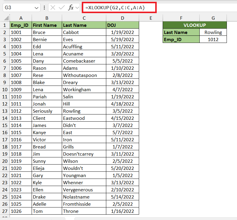
Example of Basic XLOOKUP:
This straightforward formula will look for the value in cell G2 within column C and return the corresponding value from column A.
Transitioning from VLOOKUP to XLOOKUP:
If you’re familiar with VLOOKUP, transitioning to XLOOKUP is relatively straightforward. Begin by identifying the key elements of your VLOOKUP formula and map them to the XLOOKUP function. You’ll no longer need to count columns which simplifies the process significantly.
While XLOOKUP was released for Microsoft 365 users and is not available in earlier versions, its growing popularity signals a future where Excel’s lookup functionalities are more intuitive, versatile, and robust. If your version of Excel supports it, exploring the potential of XLOOKUP can greatly improve your data management capabilities.
Best Tips for Sturdy VLOOKUP Formulas
When you rely on VLOOKUP in Excel, adopting best practices is crucial for creating sturdy formulas that provide accurate results and reduce the likelihood of errors. Here are some tips to ensure the robustness of your VLOOKUP formulas:
Use Absolute References for Table Array: Lock the table array using absolute cell references (e.g., $A$2:$C$11) to prevent it from changing when copying the VLOOKUP formula to other cells.
Keep Lookup Value Flexible: Set the lookup value as a relative reference (like E2) or lock only the column coordinate ($E2) if your table stretches across multiple rows. This allows the formula to adjust accordingly when copied down a column.
Expandable Table Arrays: To handle ranges that grow over time, convert your range into a Table with the Insert > Table command in Excel. A Table’s range will automatically expand to include new data, helping ensure your VLOOKUP always references the full dataset.
Data Validation: Use Data Validation on your lookup value cells to limit entries to a list of valid options, reducing user errors and ensuring consistent input.
Sort Data for Approximate Matches: When working with approximate matches (TRUE), ensure that your table array’s first column is sorted in ascending order. This guarantees more predictable and accurate results.
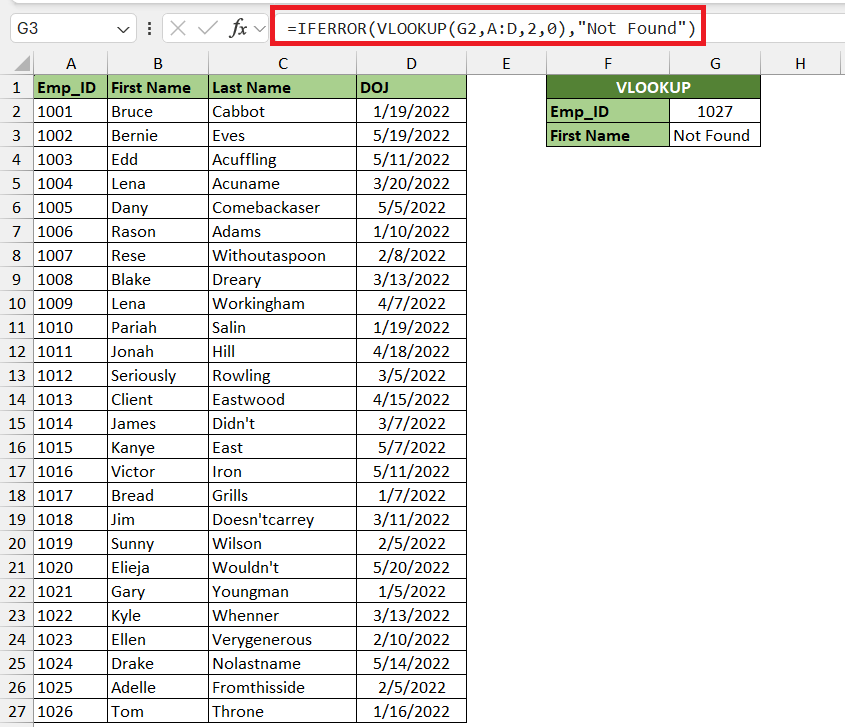
Error Handling Tactics: Implement IFERROR or IFNA to catch and manage errors like #N/A before they disrupt your workflow, allowing you to specify alternative value returns in case of an error:
Practical Helper Columns: For multiple criteria searches, utilize helper columns to concatenate the criteria into a unique identifier that VLOOKUP can use. Do not forget to mirror the concatenated formula within the VLOOKUP for the lookup_value.
Training and Efficiency: Educate users on how the VLOOKUP formula is structured and operates, so they can use it efficiently and troubleshoot it independently.
By adhering to these best practices, your VLOOKUP formulas will be more reliable, flexible, and effective in a variety of scenarios, increasing the integrity of your data analysis and decision-making processes. Remember, the time invested in setting up your VLOOKUP formulas properly pays dividends in data accuracy and user productivity.
Frequently Asked Questions
What is VLOOKUP best used for?
VLOOKUP is best used for searching for a specific value within a column and returning a value from a corresponding cell in the same row, which is a certain number of columns to the right. It’s ideal when you have a unique key, such as a name or identification number, to look up an associated piece of data, like a score or a year in a dataset.
What Settings Should I Use for Accurate VLOOKUP Results?
For accurate VLOOKUP results, you should use the exact match mode by setting the last argument in the VLOOKUP function to FALSE. Ensure the lookup value is unique and specify the correct table array range where the data is located. Additionally, check that the column number in the formula correctly corresponds to the data you want to retrieve from the table array.
How Can I Avoid Errors When Using VLOOKUP?
To minimize errors when using the VLOOKUP function in Excel, first ensure that your data is well-organized, with the lookup value being in the leftmost column of your table range. Double-check the formula for correct syntax, the right table array, and accurate sheet references. Lastly, specify the correct column index number and choose “TRUE” or “FALSE” appropriately to get an exact or approximate match based on your data setup.
What is the difference between VLOOKUP and XLOOKUP?
The primary difference between VLOOKUP and XLOOKUP is their flexibility and ease of use. VLOOKUP is limited to vertical lookups and requires the lookup value to be in the first column of the data range, returning information from columns to the right. In contrast, XLOOKUP allows for both vertical and horizontal searches, doesn’t restrict the lookup value to the first column, and is capable of returning data from any column or row, making it more versatile and less prone to errors.
John Michaloudis is a former accountant and finance analyst at General Electric, a Microsoft MVP since 2020, an Amazon #1 bestselling author of 4 Microsoft Excel books and teacher of Microsoft Excel & Office over at his flagship MyExcelOnline Academy Online Course.

