In-Cell Bar Charts with the REPT Function

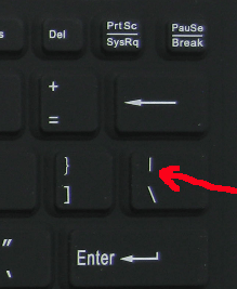
When you are creating an Excel Dashboard and are limited by space and do not want to insert a chart, you can easily create an in-cell bar chart using the REPT (repeat) function.  The REPT function uses the vertical bar character | as the first argument: text and references the value cell for the second argument: number_times. So it enters the vertical bar character by the number of times the value cell, looking something like this: ||||||||||||||||||||||||||||||||||||||||||||||||||||||||||||||||||||||||||||||||||||||||||||||

Key Takeaways

 

Introduction

What is the REPT Function?

The REPT function repeats a text string a specified number of times. The syntax of the REPT function is:

=REPT(text, number_times)

For example, if you want to insert a vertical bar in a cell 10 times, the formula will be:

=REPT(“|”,10)

Why Use In-Cell Bar Charts?

Traditional charts take up a lot of space when creating dashboards. An in-cell chart will be compact and provide instant visual comparison.

 

In-Cell Bar Charts with the REPT Function

STEP 1: Enter the REPT function in a column next to your values

=REPT(text,number_times)

STEP 2: Enter the vertical bar keyboard character in the first argument =REPT(“|”)

STEP 3: Reference the value cell for the second argument =REPT(“|”, a1)

STEP 4: Highlight the formula column, insert the Stencil font from the Home menu, and choose a font color

STEP 5: If your value cells are high, the bar will go out of your screen.  To fix this, you need to enter a divisor in the second argument of your formula, which will reduce the length, e.g., =REPT(“|”,a1/5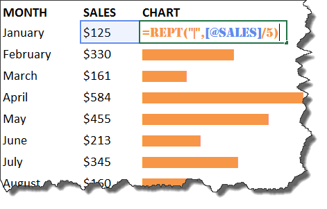

This displays one bar for every five units, keeping the chart compact while preserving the comparison.

 

Advanced Uses

Progress Bar

You can use this method to create progress bars as well. Suppose the percentage of completion is mentioned in cell B2, the formula to create a progress bar will be:

=REPT(“█”,B2/5)

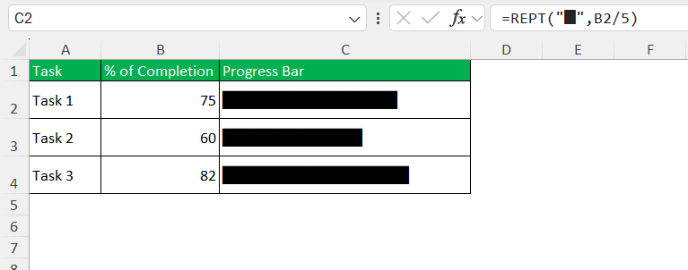
For example, a value of 75 will display approximately 15 blocks, creating a simple progress indicator.

Display Percentage

You can display both the chart and the value in the same cell using this formula:

=REPT(“█”,B2/5)&” “&B2&”%”

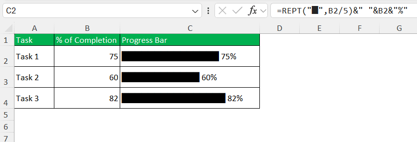
This approach works well for project tracking, task completion, and KPI dashboards.

 

Tips & Tricks

• Use Consolas or Courier New for consistent spacing.
• Scale bars relative to the maximum value for better comparisons.
• Combine REPT with TEXT to display formatted numbers.
• Add Conditional Formatting to highlight top performers.
• Use shaded characters like ░, ▒, and ▓ for professional-looking progress bars.

 

FAQs

What is the REPT function in Excel?

The REPT function repeats a specified text string a given number of times. It’s often used to create text-based visuals, like in-cell bar charts.

How do I use REPT for bar charts?

Combine a repeated character like “|” or “█” with a numeric value, e.g., =REPT("█", A1), where A1 contains the number to visualize.

How can I adjust the scale of the bar chart?

Divide each value by a factor to limit the bar length, e.g., =REPT("█", A1/10) to scale values down by a factor of 10.

Can I apply colors to in-cell bar charts?

Yes, use conditional formatting to change the font or cell color based on the value, making the bars more visually appealing.

Is the REPT bar chart better than a standard chart?

It’s not a replacement but a space-saving alternative ideal for compact views or dashboards that require minimal formatting.