Master the Power of INDEX in Excel: 2 Different Forms – Array and Reference

In this article, you will explore the following topics –

Download the Excel Workbook below to follow along and understand how to use INDEX in Excel – download excel workbookINDEX-in-Excel.xlsx

 

Introduction to Index in Excel

The INDEX function is one of the most popular tools used in Excel and is a perfect upgrade to the VLOOKUP function. It retrieves data from a specific row and column within an array. It offers the flexibility to fetch individual values, complete rows, or entire columns.

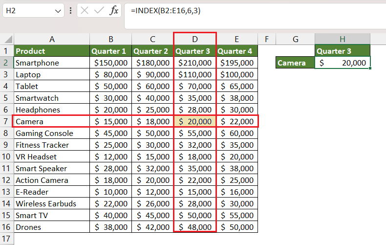
You can easily use the INDEX function When you know the row and number from which the data needs to be retrieved. For instance, if you have a sales table, and you wish to find the sales figure for Camera in Quarter 3, you can effortlessly achieve this with the INDEX Function.

No manual data search is required!

There are 2 forms in the INDEX function – array form and reference form.

Index in Array form allows input of only one range or array. Whereas, Index in Reference form will enable you to use multiple arrays along with an optional argument to specify the desired array.

Let’s explore the two different forms with examples.

 

#1 – INDEX in Array Form

Index in Array Form is a commonly used and more straightforward version. It allows you to extract values from a single table or array based on the row and column number specified by the user. The syntax is as follows –

=INDEX(array, row_num, [column_num])

• array: The range of cells or an array from which you want to retrieve data.
• row_num: The row number from which you want to extract data.
• column_num: (Optional) The column number from which you want to extract data. If omitted, INDEX will return the entire row specified by the row_num.

Let us look at an example to understand better.

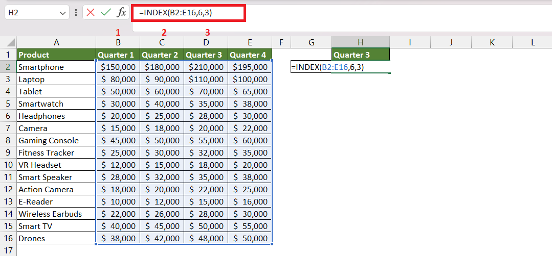
In this example, you can follow the steps below to find the sales figure for Camera in Quarter 3.

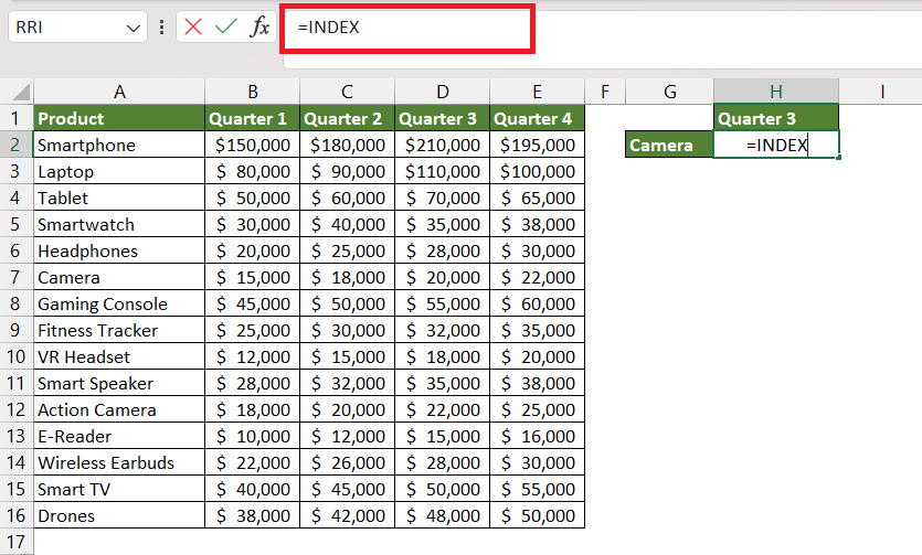
STEP 1: Enter the INDEX formula.

=INDEX

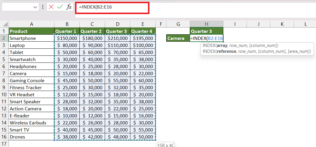
STEP 2: Enter the first argument i.e. array. This is the array that contains the lookup value. Here, it is the column containing the sales amount.

=INDEX(B2:E16

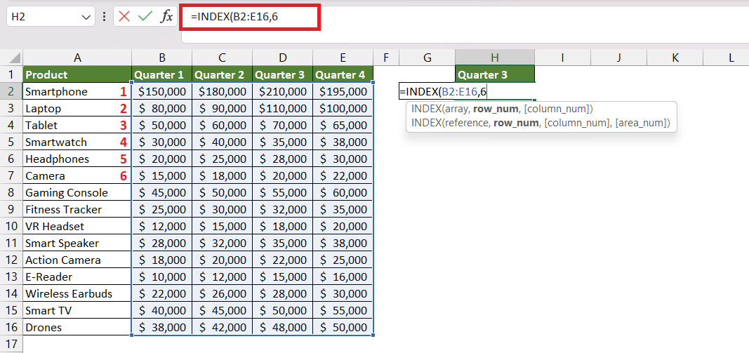
STEP 3: Enter the second argument i.e. row_num. Here, it is 6 as Camera is in the 6th row of the array B2:B16.

=INDEX(B2:E16,6

STEP 4: Enter the third argument i.e. col_num. Here, it is 3 as Quarter 3 is in the 3rd column of the array B2:B16.

=INDEX(B2:E16,6,3)

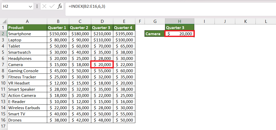
Index Function has extracted the sales figure for Camera in Quarter 3 and displayed the result i.e. $20,000.

Before you move forward, please note the following three cases that you may encounter when dealing with INDEX in Excel –

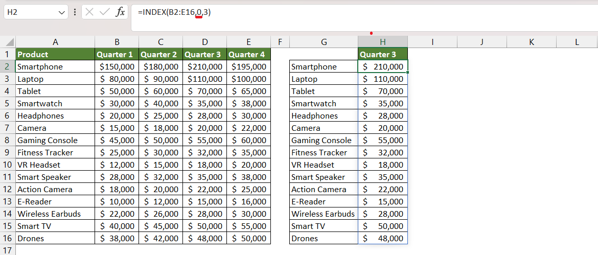
CASE 1 – If the row number is 0, Excel will return the entire column specified by the user.

=INDEX(B2:E16,0,3)

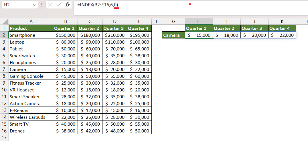
CASE 2 – If the column number is 0, Excel will return the entire row specified by the user.

=INDEX(B2:E16,6,0)

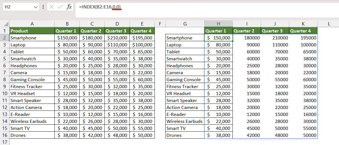
CASE 3 – If row and column numbers are 0, Excel will return the entire table.

=INDEX(B2:E16,0,0)

Here, the row and column numbers were hardcoded in the formula. If you want, you can make it dynamic by using a combination of INDEX and MATCH functions in Excel.

Instead of manually searching the position of lookup values, you can easily use the MATCH function to return the position of an item within a list or a range of cells. The syntax of the MATCH function is

=MATCH(lookup_value, lookup_array, [match_type])

where,

• lookup_value -The value you want to find within the lookup_array.
• lookup_array – The range of cells where Excel will search for the lookup_value.
• [match_type] – (Optional) This argument specifies the type of match to be performed. It can take three values:
  • 1 (or omitted) – Finds the largest value that is less than or equal to lookup_value
  • 0 – Finds the first exact match. The lookup_array must be sorted in ascending order for this to work.
  • -1 – Finds the smallest value that is greater than or equal to lookup_value. The lookup_array must be sorted in descending order for this to work.

Let us use the same example and use 2 MATCH functions to extract row and column numbers.

STEP 1: Enter the INDEX formula.

=INDEX

STEP 2: Enter the first argument i.e. array. This is the array that contains the lookup value. Here, it is the column containing the sales amount.

=INDEX(B2:E16

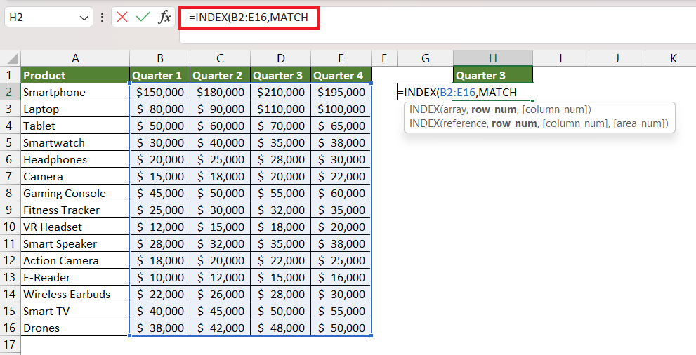
STEP 3: Enter the MATCH function.

=INDEX(B2:E16,MATCH

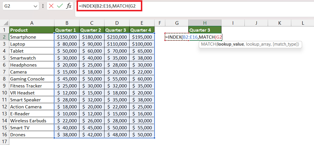
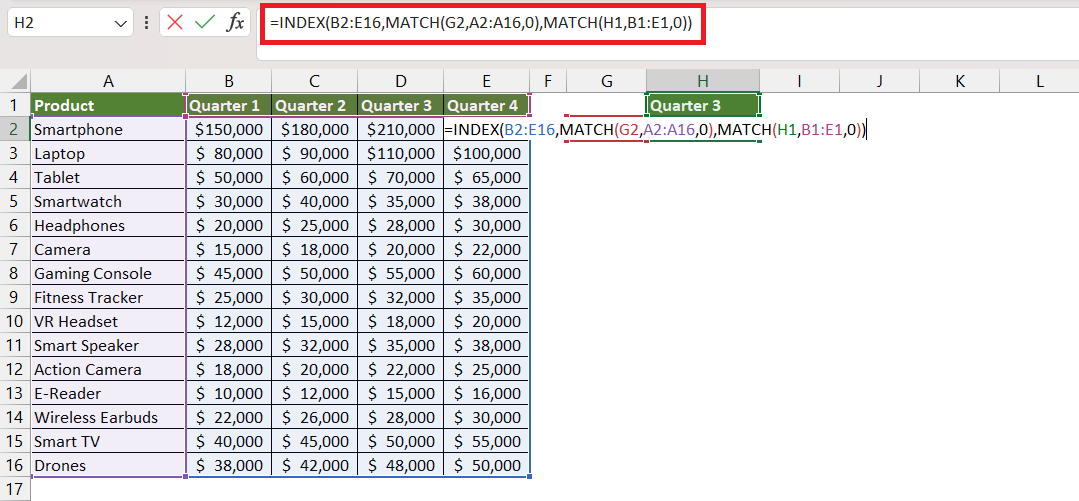
STEP 4: Enter the first argument of the MATCH function i.e. lookup_value. Here, it is Camera mentioned in cell G2.

=INDEX(B2:E16,MATCH(G2

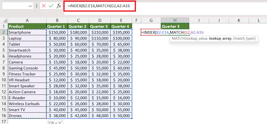
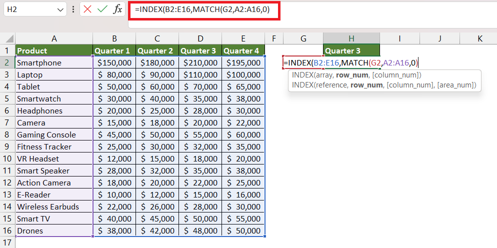
STEP 5: Enter the second argument of the MATCH function i.e. lookup_array. Here, it is the range A2:A16.

=INDEX(B2:E16,MATCH(G2,A2:A16

STEP 6: Enter the third argument of the MATCH function i.e. match_type. Here, it is 0 for an exact match.

=INDEX(B2:E16,MATCH(G2,A2:A16,0)

This MATCH function will help you in extracting the row number. Now, let us use another MATCH function to get the column number.

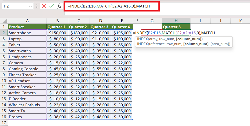
STEP 7: Enter the 2nd MATCH function.

=INDEX(B2:E16,MATCH(G2,A2:A16,0),MATCH

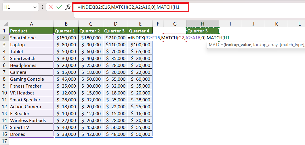
STEP 8: Enter the first argument of the MATCH function i.e. lookup_value. Here, it is Quarter 3 mentioned in cell H1.

=INDEX(B2:E16,MATCH(G2,A2:A16,0),MATCH(H1

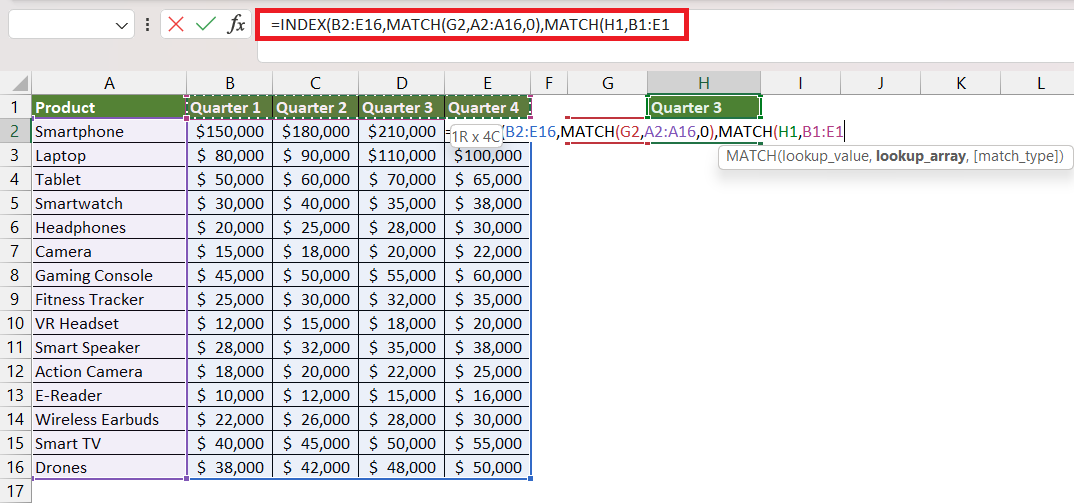
STEP 9: Enter the second argument of the MATCH function i.e. lookup_array. Here, it is the range B1:E1.

=INDEX(B2:E16,MATCH(G2,A2:A16,0),MATCH(H1,B1:E1

STEP 10: Enter the third argument of the MATCH function i.e. match_type. Here, it is 0 for an exact match.

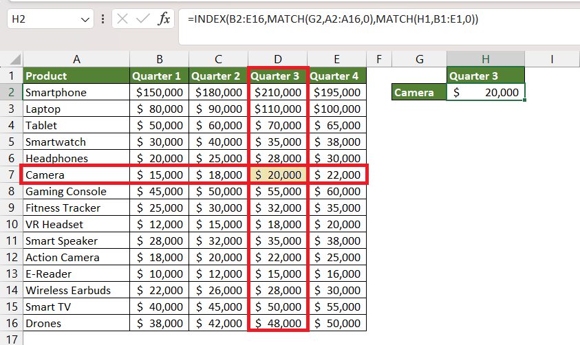
=INDEX(B2:E16,MATCH(G2,A2:A16,0),MATCH(H1,B1:E1,0))

INDEX MATCH Function has extracted the sales figure for Camera in Quarter 3 and displayed the result i.e. $20,000.

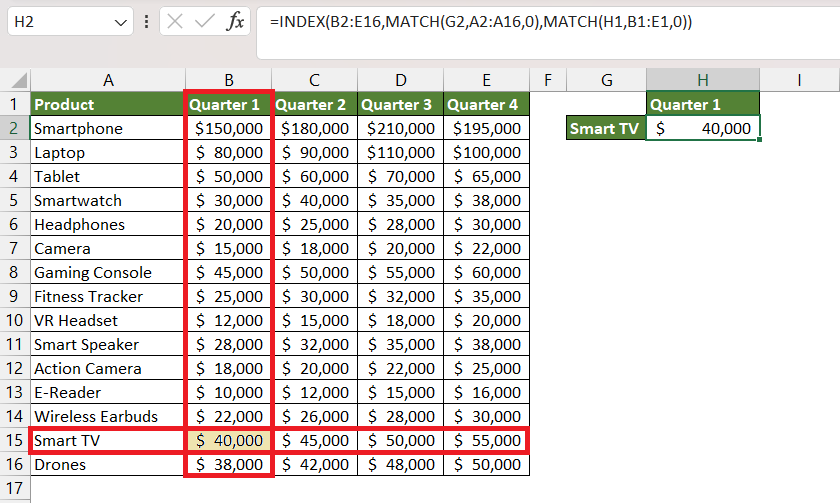
Now, let us change the values mentioned in cells G2 and H1 and see how the result changes.

 

#2 – INDEX in Reference Form

The reference form of the INDEX function takes data extraction to a whole new level by supporting multiple arrays. This form allows you to extract data from more than one range or array simultaneously, along with an optional argument to specify which array should be used.

The syntax for the reference form of INDEX is as follows:

=INDEX(reference, row_num, [column_num], [area_num] )

• reference – One or multiple ranges from which you want to extract data. Multiple ranges should be separated by commas and enclosed within parentheses.
• row_num – The row number from which you want to extract data.
• column_num (Optional) – The column number from which you want to extract data. If omitted, INDEX will return the entire row specified by the row_num.
• area_num (Optional) – The range number from which you want to retrieve data when the reference contains multiple ranges. If omitted, INDEX will return the result from the first range.

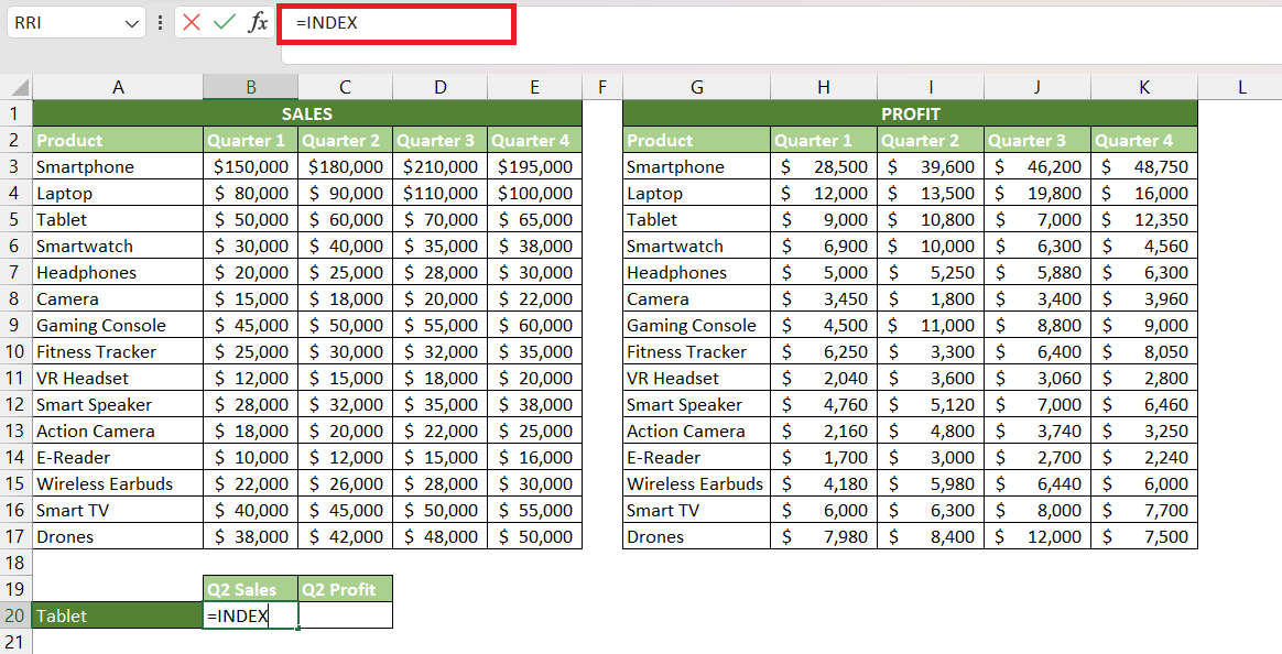
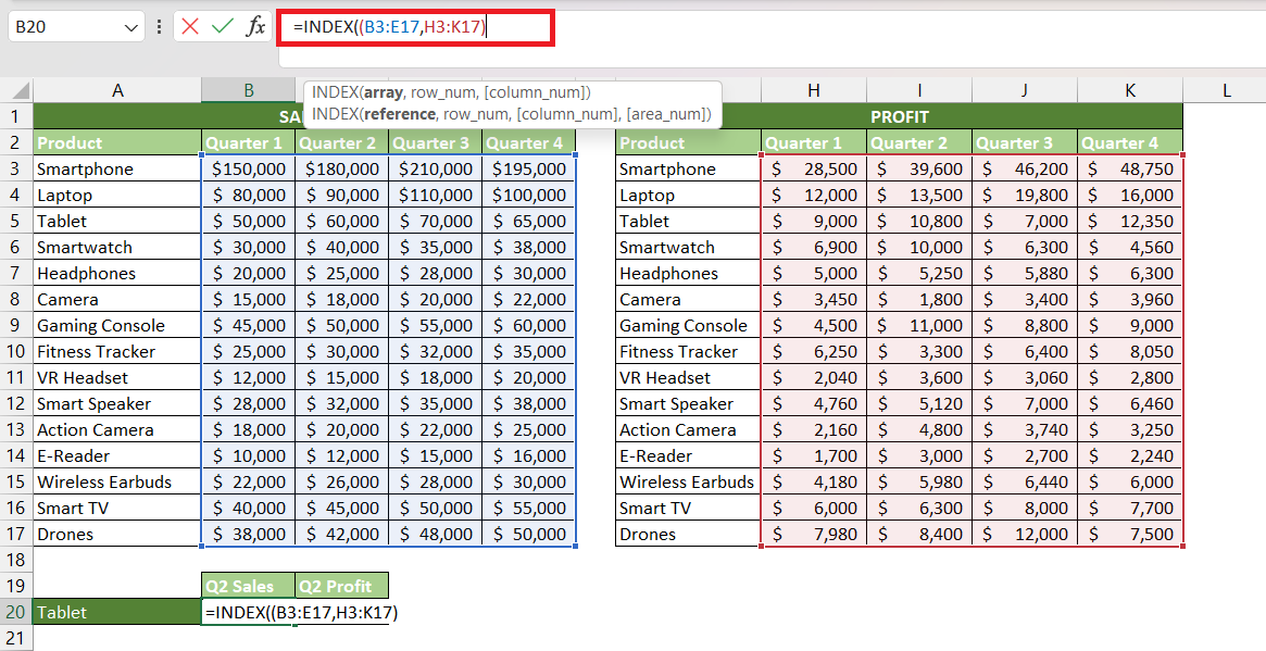
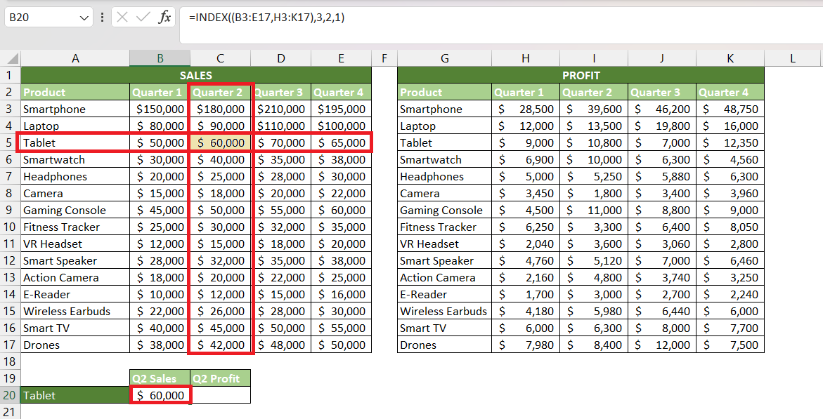
Suppose, there are two datasets – one containing quarterly sales figures for products and another with corresponding profit values. Now, let us use INDEX in reference form to extract values.

To extract sales figures for Tablet in Quarter 2, follow the steps below –

STEP 1: Enter the INDEX formula.

=INDEX

STEP 2: Enter the first argument i.e. reference. Here, it is both the ranges containing sales and profit values separated by commas and enclosed in parenthesis.

=INDEX((B3:E17,H3:K17)

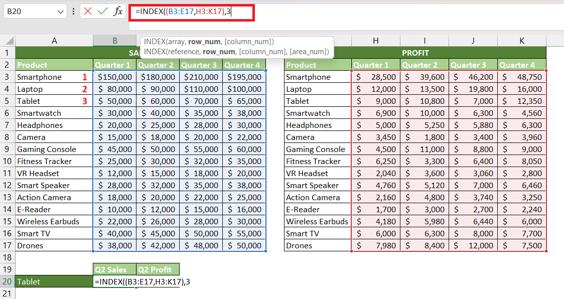
STEP 3: Enter the second argument i.e. row_num. Here, it is 3 as Tablet is in the 3rd row.

=INDEX((B3:E17,H3:K17),3

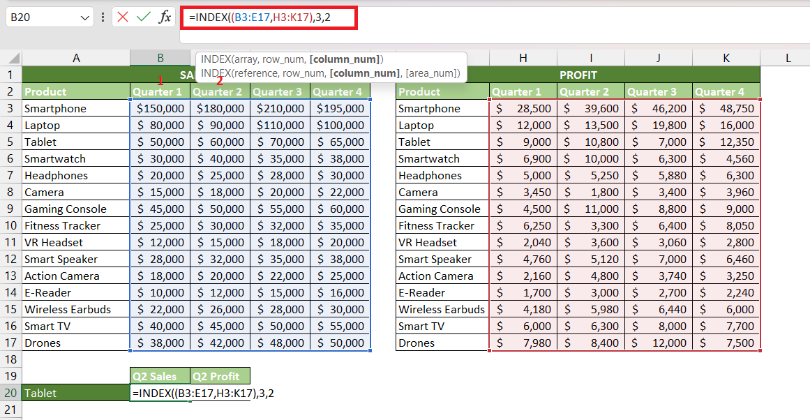
STEP 4: Enter the third argument i.e. col_num. Here, it is 2 as Quarter 2 is in the 2nd column of the array.

=INDEX((B3:E17,H3:K17),3,2

 

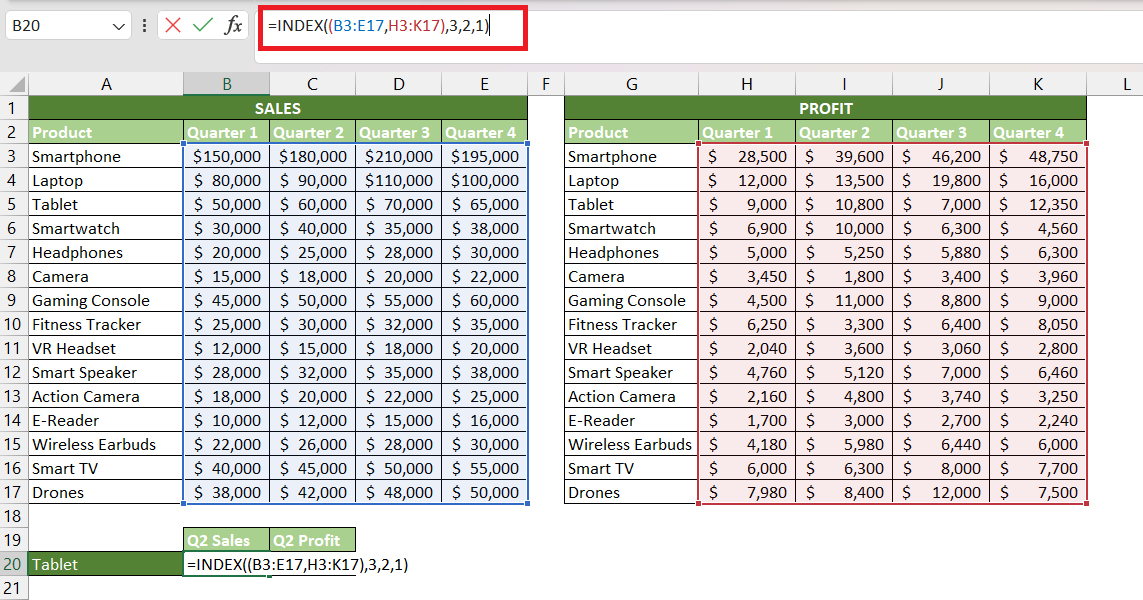
STEP 5: Enter the fourth argument i.e. area_num. Here, it is 1 as sales figures are mentioned in the 1st array i.e. B3:E17.

=INDEX((B3:E17,H3:K17),3,2,1)

Index Function has extracted the sales figure for Tablet in Quarter 2 and displayed the result i.e. $60,000.

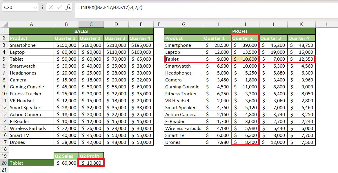
Similarly, if you want to display the profit amount you need to insert the area_num. This is because profit values are mentioned in the 2nd array of the reference i.e. H3:K17.

 

Conclusion

This article discusses INDEX in Excel, focusing on its two forms: array and reference. The array form allows the extraction of data from a single array, while the reference form extends this capability to multiple arrays.

This function makes data manipulation in Excel more efficient and accurate.

Click here to learn more about INDEX in Excel!