Table of Contents
Introduction to Powerful Excel Lookups
The Era of Traditional Lookup Functions
Traditional Excel lookup functions like VLOOKUP were once the go-to tools for finding data. With them, users were able to search for a piece of data within a column and retrieve information from another column in the same row. However, these traditional lookup functions did come with limitations, particularly when it came to looking up values in columns to the left or handling large datasets efficiently.
Embracing the INDEX MATCH Combo
Say goodbye to the limited reach of traditional lookups and hello to their more dynamic and capable successor—the INDEX MATCH combo. The amalgamation of these two functions opens up a world of possibilities, allowing you to look across rows and columns in any direction. This power duo doesn’t discriminate based on data layout, inviting you to unleash your Excel potential without the earlier constraints that sometimes led to creative but convoluted solutions.
Why INDEX MATCH Outshines VLOOKUP
Versatility Across Rows and Columns
INDEX MATCH is like a Swiss Army knife for data lookups, offering amazing versatility across rows and columns that VLOOKUP can hardly match. With this dynamic duo, you’re no longer restricted to rightward searches from the leftmost column. They empower you to traverse left, right, up, and down, effortlessly matching data in any direction you need. This is particularly useful when your data isn’t structured perfectly or when the columns you’re referencing might shift over time.
Performance Efficiency in Large Data Sets
In a showdown of efficiency, INDEX MATCH often comes out on top, especially with large datasets. Unlike VLOOKUP, which can slow down your workbook as it sifts through every row until the correct one is found, INDEX MATCH is nimbly designed to pinpoint the exact location of your desired data. This results in faster calculations and ultimately, a more performance-efficient spreadsheet experience. Less waiting time means more productivity for you.
Getting Started with INDEX MATCH
Understanding the Syntax and Parameters
Diving into INDEX MATCH is like learning a new language, but once you get the syntax and parameters down, you’ll be speaking fluently in no time. Here’s the gist: INDEX function returns the value of a cell in a specific row and column within a range,
=INDEX(array, row_num, [column_num])
What it means:
=INDEX(from this table/range, return me this row number, [and return me this column number])
While the MATCH function provides the position of a lookup value within a range.
=MATCH(lookup_value, lookup_array, [match_type])
What it means:
=MATCH(lookup this value, from this list or range of cells, return me the Exact Match)
INDEX and MATCH are separate functions that complement each other:
- INDEX function: Returns the value of a cell in a table based on the row and column number.
- MATCH function: Searches for a specified value in a range and returns its relative position.
=INDEX(array, MATCH(lookup_value, lookup_array, [match_type])
What it means:
=INDEX(return the valu qe/text, MATCH(from the row position of this value/text))
Think of INDEX as saying “Go to this row and column,” and MATCH as saying “The data you want is located here in this position.
Preparing Your Excel Workbook for Index Match
Before setting your sights on mastering INDEX MATCH, a little groundwork is necessary. Preparing your Excel workbook will save you from headaches down the line. Begin by ensuring your data is neatly organized, with clear headers and no blank rows or columns interrupting your ranges.
Additionally, make sure your lookup values are unique to avoid mismatches – think of it as setting the stage for a flawless performance by INDEX MATCH.
Step-by-Step Easy Tutorial on Using INDEX MATCH
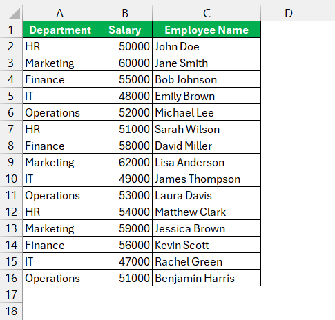
Let’s use INDEX MATCH to find out the salary of “Rachel Green”.
STEP 1: Using MATCH to find the row number
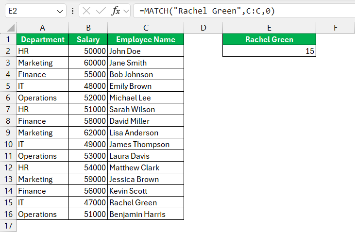
=MATCH(“Rachel Green”, C:C, 0)
In this formula:
- “Rachel Green” is the lookup value you want to find in column C (Employee Name).
- C:C specifies the lookup array where Excel will search for the lookup value.
- 0 specifies that you want an exact match.
Assuming “Rachel Green” is found in row 15, MATCH will return 15 as the result.
STEP 2: Using INDEX to retrieve the corresponding salary
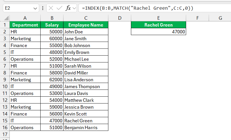
=INDEX(B:B,MATCH(“Rachel Green”, C:C, 0)
In this formula:
- B:B specifies the range from which Excel will return the result (column B, where salaries are listed).
- MATCH(“Rachel Green”, C:C, 0) returns 1,5 which is the row number where “Rachel Green” is located in column C.
INDEX then retrieves the value in column B that corresponds to the row number returned by MATCH.
Therefore, if “Rachel Green” corresponds to row 15 in column C and her salary is in row 15 of column B, the formula will return 47000 as a result.
Real-Life Scenarios: Applying INDEX MATCH in Business Challenges
Extracting Specific Data from Sales Reports
When tackling dense sales reports, the INDEX MATCH function acts as your personal data miner. Imagine an expansive spreadsheet with rows of products, and columns with sales data from various periods and regions. With INDEX MATCH, you can easily extract the exact sale figures for a specific product at a specific time in a specific region. No more endless scrolling; just precise, efficient data extraction that allows you to make informed business decisions swiftly.
Managing Inventory with Two-Way Lookups
Inventory management can be complex, but with two-way lookups using INDEX MATCH, it becomes a breeze. This technique lets you search for an item horizontally across the column headers and vertically along the row labels, meeting in the middle at the exact stock level you require. Quick updates on inventory levels across multiple categories become so intuitive, it’s almost like having an extra pair of hands handling the data for you.
Additional Example in Getting the Stock ID
We want to get the stock id of the tablet, and we will use a combination of INDEX and MATCH to get this!
STEP 1: We need to enter the INDEX function in a blank cell:
=INDEX(
STEP 2: The INDEX arguments:
Array
Where is the list that contains the stock ids?
=INDEX(B13:B17,
Row_num
What row number contains the data?
Let us use the Match function to get the row number.
=INDEX(B13:B17, MATCH(
STEP 3: The MATCH arguments:
Lookup_value
What is the value that we want to match?
We want to match the Tablet.
=INDEX(B13:B17, MATCH(G14,
Lookup_array
Where is the list that contains the stock items?
=INDEX(B13:B17, MATCH(G14, C13:C17,
Match_type
What kind of matching do you want?
Let’s put in 0 to get the exact match
=INDEX(B13:B17, MATCH(G14, C13:C17, 0))
With this, the MATCH function will get the row number containing the Tablet, which is row #3. Then with Row #3, we will get the stock id in that same row using the INDEX function.
Two-way lookup with INDEX and MATCH
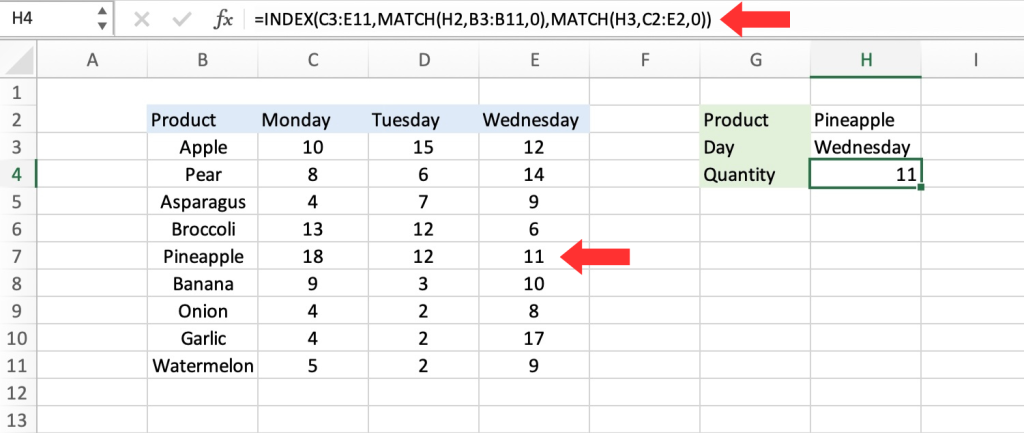
Is there a way to create a completely flexible formula that can return data for any product in any day? To achieve this, we need to use MATCH twice: one to determine the row position and the other to determine the column position.
Based on the examples provided, it is evident that MATCH works effectively with arrays in both horizontal and vertical orientations. This implies that locating the position of a specified month using MATCH is a simple task. To illustrate, the following formula identifies the position of Wednesday, which is 3:
=MATCH(“Wednesday”, C2:E2,0) // returns 3
Naturally, it is preferable not to hardcode values. Therefore, let us modify the worksheet to enable the input of a day’s name and utilize MATCH to locate the relevant column number:
=INDEX(C3:E11,MATCH(H2,B3:B11,0),MATCH(H3,C2:E2,0))
After the initial MATCH formula returns 5 to INDEX as the row number, and the second MATCH formula returns 3 to INDEX as the column number, the formula is simplified to:
=INDEX(C3:E11,5,3)
and INDEX correctly returns 11, the quantity of Pineapples sold on Wednesday.
Left Lookup
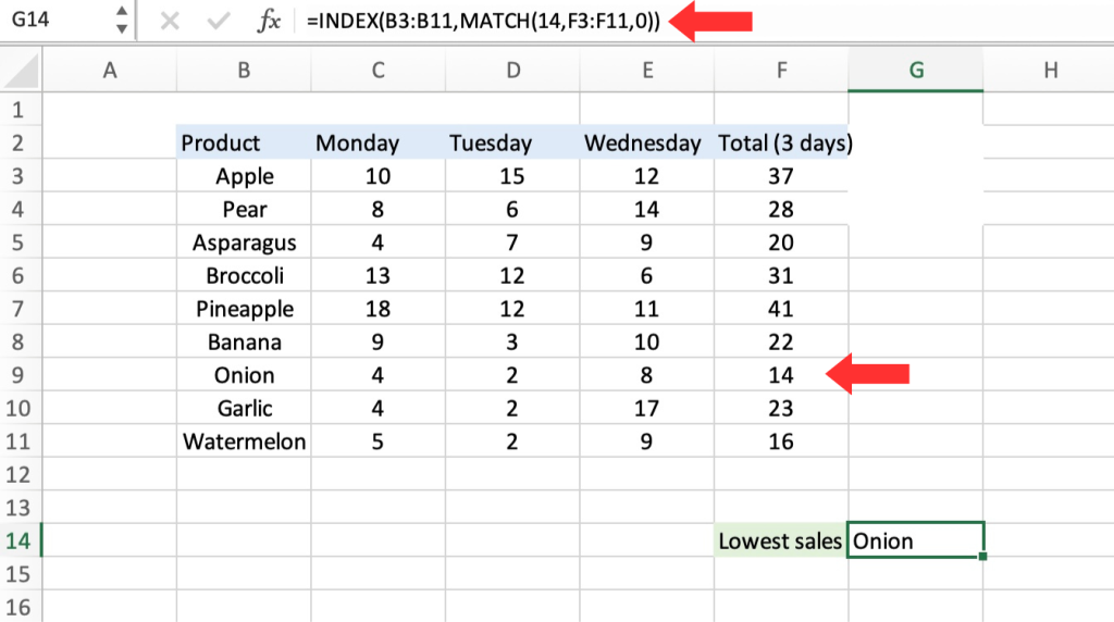
INDEX and MATCH offer a significant advantage over the VLOOKUP function, which is the capability to perform a “left lookup.” Essentially, this refers to a search in which the identifier column is located to the right of the values that require retrieval:
=INDEX(B3:B11,MATCH(14,F3:F11,0))
We can easily find out the onion’s total sales by using the VLOOKUP function. The left LOOKUP is the opposite of that. If we wanted to find out which product got the lowest amount of sales (14), it would lead to the onion.
Case-sensitive Lookup
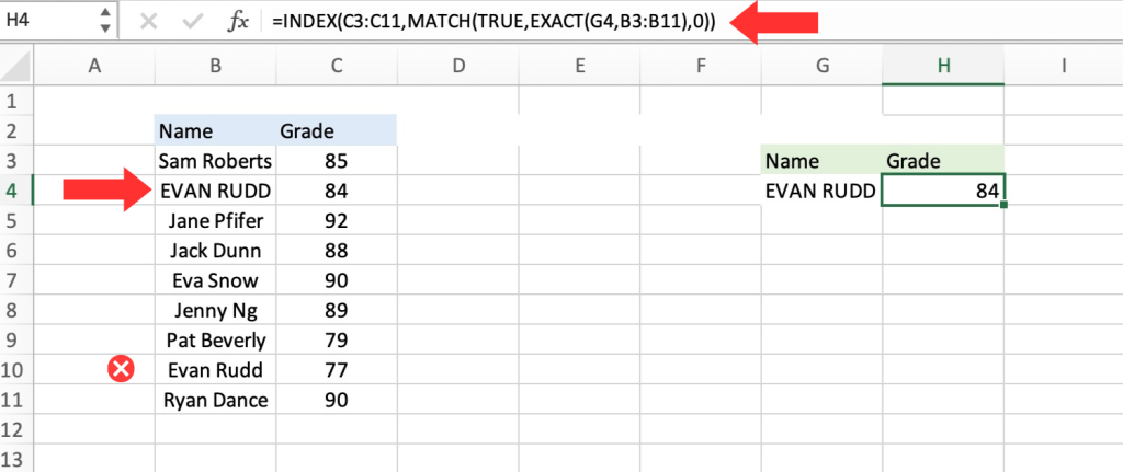
Although the MATCH function does not consider the case sensitivity, you can incorporate the EXACT function along with INDEX and MATCH to carry out a lookup that takes into account the upper and lower case, as demonstrated below:
=INDEX(C3:C11,MATCH(TRUE,EXACT(G4,B3:B11),0))
Common Pitfalls and How to Avoid Them
Dealing with Error Values in INDEX MATCH
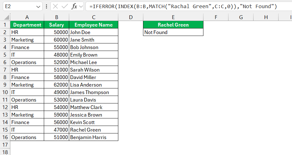
Even the best-laid INDEX MATCH formulas can encounter errors, leaving you staring at an unhelpful #N/A. Fear not, for these can be tamed with functions like IFNA and IFERROR. Wrap your formulas with these safeguards to catch and clarify errors, such as indicating a missing match.
Remember, though, while IFERROR can conceal all errors, using it indiscreetly might hide valuable clues about any mistakes in your setup, so use it judiciously.
Ensuring Accurate Matches with Data Types and Formatting
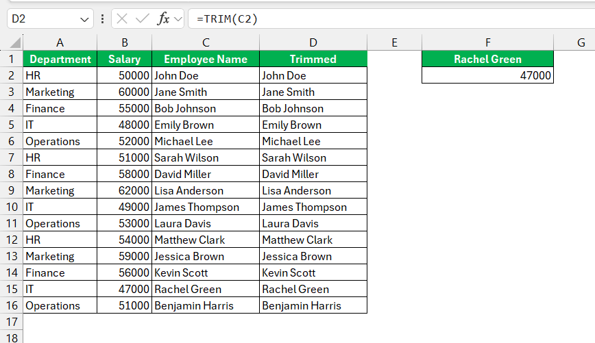
Accuracy in INDEX MATCH lookups is paramount, and it stands on the foundation of consistent data types and formatting. Ensure your lookup values and the data in the table you’re searching through match in type—text with text, numbers with numbers. Pay attention to extra spaces or non-printable characters that may slip into your data, as they can skew your results. Using functions like TRIM or CLEAN helps to maintain a squeaky-clean dataset, primed for spot-on matches.
FAQs: Your Questions Answered
How do I use an INDEX match in Excel?
To use an INDEX MATCH in Excel, follow these steps: First, type =INDEX( and select the range that has the value you want to return. Next, add a comma, then MATCH( and select your lookup value. After another comma, choose the range to search for the lookup value. Close the MATCH function with ), add the matching column or row for the index range, close with ), and hit Enter.
Can I Use INDEX MATCH for Left Lookups?
Absolutely! Unlike VLOOKUP, with INDEX MATCH you’re not constrained to looking from left to right. To do a left lookup, just set the return range in the INDEX function to the left of the match range in the MATCH function. It’s a straightforward way to pull data from columns that are to the left of your lookup value.
How Does INDEX MATCH Perform with Unsorted Data?
INDEX MATCH performs admirably with unsorted data—it doesn’t require data to be in any specific order to find the correct match. This sets it apart from lookup functions that depend on sorted data, offering flexibility and simplicity in data retrieval, regardless of how your data is arranged.
Are There Any Limitations to INDEX MATCH?
Even though INDEX MATCH is a robust and flexible tool, it does have limitations. It can become complex and require more processing power with very large datasets or complex, nested usage. Additionally, users need to understand its syntax and how to manipulate arrays, which might be challenging for beginners. As with any Excel function, accuracy also depends on correct data input and avoidance of errors in your formulas.
What Alternatives Exist to INDEX MATCH for Complex Lookups?
For complex lookups, you might consider using XLOOKUP, a new function designed to overcome the limitations of both VLOOKUP and INDEX MATCH. XLOOKUP offers a simplified syntax, defaults to exact match lookups, and can search in both directions. Another alternative is the combination of SUMIFS, COUNTIFS, and AVERAGEIFS for lookups that require summing, counting, or averaging data based on multiple conditions.
John Michaloudis is a former accountant and finance analyst at General Electric, a Microsoft MVP since 2020, an Amazon #1 bestselling author of 4 Microsoft Excel books and teacher of Microsoft Excel & Office over at his flagship MyExcelOnline Academy Online Course.

