How to use LINEST function in Excel

Excel has several built-in statistical functions that help analyze and summarize data. The LINEST function in Excel is used to calculate the statistics for a line that best fits your data. This is often referred to as linear regression or trendline analysis.

In this article, we will cover the following in detail –

Download the Excel Workbook below to follow along and understand How to use the LINEST function in Excel –

download excel workbookLINEST-Function.xlsx

What is Linear Regression

Before we dive into the LINEST function, let us first understand what is linear regression.

Linear regression is a statistical method used to model the relationship between a dependent variable and one or more independent variables by fitting a linear equation to the observed data. The key assumption is that the relationship between the variables can be approximated by a straight line.

The general form of a simple linear regression equation with one independent variable is:

y = mx + b

Here:

• y is the dependent variable.
• x is the independent variable.
• m is the slope of the line, which represents the change in y for a unit change in x.
• b is the y-intercept, the value of y when x is 0.

Introduction to LINEST function

The LINEST function in Excel is a statistical tool that employs the “least squares” method to compute the statistics for a line. It does this by determining a straight line that optimally fits your data, minimizing the sum of squared differences between observed and predicted values. The syntax of this function is as follows –

LINEST(known_y’s, [known_x’s], [const], [stats])

where,

• known_y’s – This is the array or range of dependent variables (y-values) in your data.
• known_x’s – This is an optional argument. It is the array or range of independent variables (x-values) in your data. If omitted, Excel assumes the x-values are 1, 2, 3, …, n.
• const – This is an optional argument.
  • If const is TRUE or omitted, the LINEST function includes an intercept in the model. The equation will be y = mx + b
  • If const is FALSE, the function assumes there is no intercept. The equation will be y = mx.
• stats – This is an optional argument.
  • If stats is TRUE, the LINEST function returns additional regression statistics.
  • If stats is FALSE or omitted, only the coefficients of the line are returned.

Since this function returns an array of values, it enters to be entered as an array function as well. Please remember to press Ctrl +  Shift  + Enter after writing all the arguments of this function.

Example of LINEST function

Who doesn’t love video games?!! Now we all know that more the hours put into a game, the higher will be the results. Your progress is tracked by your score, which directly corresponds to how much you practice.

When linking two variables, regression analysis can be used to determine how much of an impact one variable has on the other. This means that regression can help us calculate how much your score will increase for each additional hour of gameplay. Let’s understand 2 foundational aspects of regression:

y = mx + b

• y – It is the score you get.
• x – It is the number of hours you put in.
• b – It is the intercept. Picture it as a starting point. Even if you didn’t play at all, you might still have a base score.
• m – It is the slope. It tells you how much your score changes for each hour you play. If the slope is high, your score jumps a lot with each hour. If it’s low, the increase is smaller.

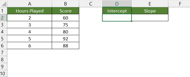
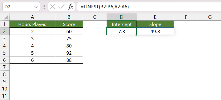
Here is the data set for this example –

Follow the steps below to use the LINEST function to get the slope and intercept for this example –

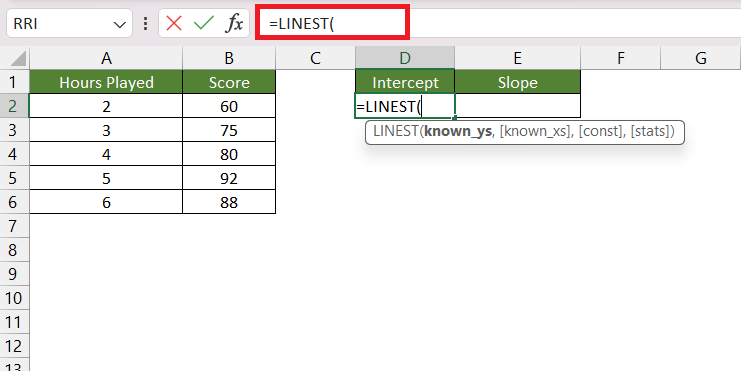
STEP 1: Enter the LINEST function.

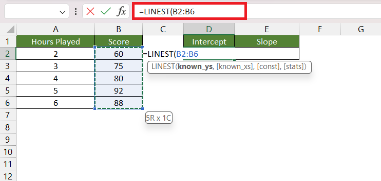
STEP 2: Enter the first argument i.e. known_y’s. Here, is the list containing the scores.

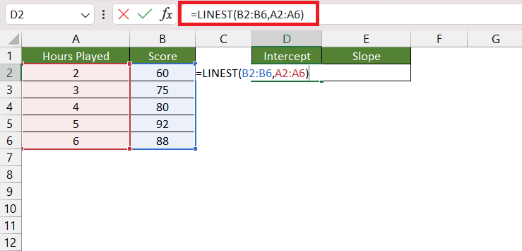
STEP 3: Enter the second argument i.e. known_x’s. Here, is the list containing the hours played.

STEP 4: Press Ctrl + Shift + Enter.

You will see that Excel will provide you with two values. The first one is the slope i.e. 7.3 and the second is the intercept i.e. 49.8.

The equation that will be formed using these values is –

y = 7.3x + 49.8

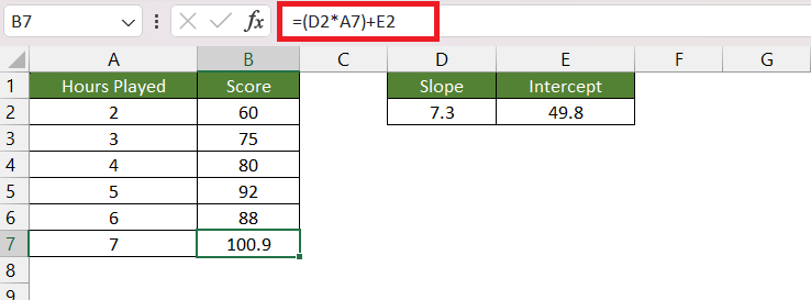
Now, let us add another row with the number of hours played as 7 and use this equation to get the probable score.

The score will be around 101.

Conclusion

The article discusses the use of the LINEST function in Excel for linear regression analysis. Linear regression is explained as a statistical method to model the relationship between a dependent variable and one or more independent variables by fitting a linear equation to observed data. The LINEST function, employing the least squares method, calculates the statistics for a line that best fits the data and returns an array describing the line, including slope and intercept.

Click here to learn more about the LINEST function.

If you like this Excel tip, please share it

email

Pinterest

Facebook

Twitter

Linkedin

John Michaloudis

Founder & Chief Inspirational Officer at MyExcelOnline.com

John Michaloudis is a former accountant and finance analyst at General Electric, a Microsoft MVP since 2020, an Amazon #1 bestselling author of 4 Microsoft Excel books and teacher of Microsoft Excel & Office over at his flagship Academy Online Course.