Table of Contents
Pivot Table Calculated Item
Pivot Table Calculated Items allow you to do mathematical calculations with your Item List. You can use any of the Excel mathematical equations, like /*+-%.
The only limitation is that you cannot reference any cells. Pivot Table Calculated Items can be used to calculate changes between each other, like a month´s or year’s value, averages or summation.
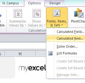
To activate the Calculated Item you have to make sure that you click on the chosen Item in the Pivot Table, then go to the PivotTable Tools tab in the Ribbon and go to Options > Fields, Items & Sets > Calculated Item.
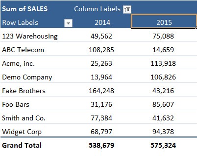
STEP 1: Click on the item that you want to calculate.
STEP 2: Click on the Pivot Table and Go to Options > Fields, Items, & Sets > Calculated Item
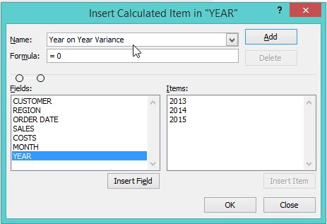
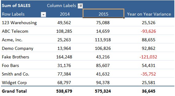
STEP 3: Set the Name to Year on Year Variance
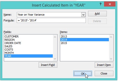
STEP 4: Set the Formula to use the Years: ‘2015’-‘2014’. Click OK.
Your Calculated Item is now ready!
John Michaloudis is a former accountant and finance analyst at General Electric, a Microsoft MVP since 2020, an Amazon #1 bestselling author of 4 Microsoft Excel books and teacher of Microsoft Excel & Office over at his flagship MyExcelOnline Academy Online Course.

