VLOOKUP formula is primarily used to look for a value in the leftmost column of the table and return the corresponding value from another column on the right.
What if you want to VLOOKUP multiple columns at once? You can use Excel VLOOKUP multiple columns by using an Array Formula! Without further ado let's dive into these topics and understand how to use VLOOKUP for multiple columns! As this is an array formula, to make it work we simply need to press CTRL+SHIFT+ENTER at the end of the formula.A very powerful feature for any serious analyst!
Excel VLOOKUP Multiple Columns Syntax
What does it do?
Searches for a value in the first column of a table array and returns the sum of values in the same row from other columns (to the right) in the table array.
Formula breakdown:
{=SUM(VLOOKUP(lookup_value, table_array, {col_index_num1,col_index_num2}, [range_lookup]))}
What it means:
{=SUM(VLOOKUP(this value, in this list, {and sum the value in this column, with the value in this column}, Exact Match/FALSE/0]))}
Now that you are familiar with the syntax let’s look at an example of how to use Excel VLOOKUP multiple columns!
Return Multiple Values
One of the downsides of using VLOOKUP is that it can return value from a single column only.
In this example, we want to find a match for both Item Description and Price. But it won’t be possible to use the basic VLOOKUP syntax.

You can modify the VLOOKUP formula with an array formula and extract both description and price by matching the item code!
Follow the step-by-step tutorial on how to VLOOKUP for multiple sheets with example and download this Excel workbook to practice along:
STEP 1: Select the cells (H8 and I8) where you want to insert the values from multiple columns.

STEP 2: We need to enter the VLOOKUP function in the selected cell:
=VLOOKUP(

STEP 3: We need to enter the first argument – Lookup_value
What is the value to be looked up?
Select the cell that contains the item name, which is cell G8.
=VLOOKUP(G8,

STEP 4: We need to enter the second argument – Table_array
Where is the list of data?
Select the Inventory table, as that is where our formula is going to get both description and price for different item codes.
Make sure you freeze the range by pressing F4!
=VLOOKUP(G15,$B$6:$D$17,

STEP 5: We need to enter the third argument – {Col_index_num1, Col_index_num2}
Which columns in the table_array contain the data you want to return?
We want to get the description and price. So that will be columns 2 and 3.
=VLOOKUP(G8, $B$6:$D$17, {2,3},

STEP 6: We need to enter the fourth argument – [Range_lookup]
Would it be an approximate match?
Set this to FALSE or 0 as we want an exact match for the Item code.
=VLOOKUP(G8, $B$6:$D$17, {2,3}, 0)

STEP 7: Press Ctrl + Shift + Enter at the end of the formula to change it into an array function.

Copy-Paste this formula for the remaining item codes mentioned in the Invoice!

Return Sum of Multiple Values
The VLOOKUP function can be combined with other functions such as the Sum, Max, or Average to calculate values in multiple columns. As this is an array formula, to make it work we simply need to press CTRL+SHIFT+ENTER at the end of the formula. A very powerful feature for any serious analyst!
See how easy it is to implement in less than 1 minute with this VLOOKUP for multiple columns example!
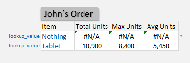
We want to get the total number of units for Laptop (16,700 + 18,700 units).
STEP 1: We need to enter the VLOOKUP function in a blank cell:
=VLOOKUP(

STEP 2: The VLOOKUP arguments:
Lookup_value
What is the value to be looked up?
Select the cell that contains the item name, which is Laptop.
=VLOOKUP(G15,

Table_array
Where is the list of data?
Select the Units Sold table, as that is where our formula is going to get the unit numbers.
=VLOOKUP(G15, B14:D17,

{Col_index_num1, Col_index_num2}
Which columns in the table_array contain the data you want to return?
We want to get the unit numbers of Years 2013 and 2014. So that will be columns 2 and 3.
=VLOOKUP(G15, B14:D17, {2,3},

[Range_lookup]
Would it be an approximate match?
Set this to FALSE as we want an exact match for Laptop.
=VLOOKUP(G15, B14:D17, {2,3}, FALSE)

STEP 3: Now wrap the formula with the SUM formula as we want to get the total number of sold units for Laptop.
=SUM(VLOOKUP(G15, B14:D17, {2,3}, FALSE))
Ensure you are pressing CTRL+SHIFT+ENTER as we want to calculate this as an array formula.

Do the exact same formula for Max Units and Average Units, by changing the SUM Formula with the MAX Formula and Average Formula respectively.

Troubleshooting Common VLOOKUP Issues
Solving Problems with VLOOKUP on Rows and Columns
When your VLOOKUP is misbehaving, it may be due to mismatches between the layout of your lookup value and the table array you’re querying. VLOOKUP traditionally searches for a value in the first column of a table and returns a result from the same row in a specified column. If your data isn’t arranged accordingly or contains merged cells or hidden rows, VLOOKUP might return incorrect results or errors.
To solve issues with rows and columns, first check that your rows are consistent and that your VLOOKUP’s range starts with the column containing your lookup value. Secondly, ensure that there are no merged cells in your table array since VLOOKUP can’t handle them properly.
For a smoother experience, ensure your data is clean, the lookup column is sorted if you’re not performing an exact match, and the column index number correctly corresponds to the column from which you want to retrieve the value.
Quick Fixes:
- Re-arrange the data ensuring the lookup column is the first column in your table array
- Remove any merged cells within your search area
- Use absolute cell references to lock down your array range
Common Pitfalls:
- Incorrectly counting columns leading to wrong column index numbers
- Overlooking leading, trailing, or hidden spaces in your data that affect lookups
For Whom It’s Best:
This remedy is for anyone who’s been frustrated by the “#N/A” or “#REF!” errors VLOOKUP throws up. It’s perfect for analysts, office administrators, and anyone else who relies on large spreadsheets for their daily tasks and requires accurate data retrieval across rows and columns.
Dealing with Errors and Inconsistencies
Encountering errors and inconsistencies when using VLOOKUP can be a common frustration. However, they can often be easily resolved with a few checks and tweaks. For example, if VLOOKUP returns the dreaded “#N/A” error, it could mean the lookup value doesn’t exist in the table array. Make sure there are no discrepancies, such as leading or trailing spaces or case sensitivity issues that might be causing a mismatch.
Another common issue is the “#VALUE!” error, usually a result of an incongruity between the data formats or an incorrect column index number. Ensuring consistency in the format of lookup values and the corresponding table array values is key – numbers should match numbers, text should match text, and so on.
Balancing the VLOOKUP formula to avoid errors involves double-checking every aspect, from ensuring the table array is not missing the lookup value column to confirming that the range lookup value is set correctly (TRUE for an approximate match or FALSE for an exact match).
Remember, an ounce of preemptive checking can save you a ton of time troubleshooting!
Proactive Strategies:
- Regular data cleansing to maintain consistency
- Using TRIM and UPPER/LOWER functions to ensure text uniformity
- Verifying formats and index numbers are correct
Potential Setbacks:
- Failure to diagnose the correct source of the error
- Inadvertent changes in the data array caused by row or column insertions
Who Benefits Most:
Anyone who regularly uses VLOOKUP for data lookups, especially in environments where data is frequently updated or altered. Ideal for professionals in roles like data analysis, accounting, or inventory control, where accuracy is crucial, and errors can be costly.
VLOOKUP Best Practices and Efficiency Tips
How to Optimize Your VLOOKUP Workflow
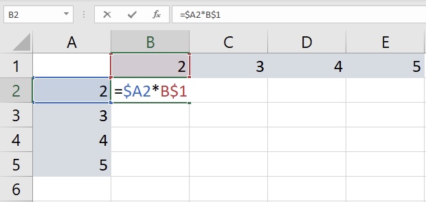
Optimizing your VLOOKUP workflow is all about using the function efficiently to save time and reduce errors. Start by ensuring your lookup table is well-organized, with unique identifiers in the first column for an unambiguous search. It’s also crucial to use absolute cell references (dollar signs in cell addresses) to prevent references from shifting if you copy and paste your formula elsewhere.
To enhance efficiency, minimize full-column references, which can slow down Excel by unnecessarily searching blank cells. Instead, define the specific range or use dynamic named ranges. Additionally, consider sorting your table array data if you are using approximate match lookup—this can significantly speed up search times.
To further streamline your workflow, use helper columns to preprocess data—especially when dealing with multiple criteria. This preprocessing can simplify what you’re asking VLOOKUP to do, leading to cleaner and more manageable formulas.
Remember, incorporating these little tricks into your daily routine not only sharpens your productivity but also ensures you’re delivering accurate outcomes in your data tasks.
Main Steps:
- Organize data with a clear, unique identifier in the first column
- Always use absolute cell references to maintain cell relation
- Limit your lookup range to only the necessary cells
Potential Hurdles:
- Adjusting habits to include these optimizations in normal workflow
- Initial time investment to set up dynamic ranges or helper columns
Who Benefits Most:
This optimization strategy is a must-have for someone who relies heavily on VLOOKUP in their job, such as data analysts or financial accountants. Consistent use of these tactics can lead to a smoother, more reliable, and ultimately more productive Excel experience.
Frequently Asked Questions on VLOOKUP Multiple Columns
Can I use VLOOKUP to return multiple columns?
Certainly! To retrieve multiple columns, you can replicate the VLOOKUP formula across different cells, modifying the column index number in each to correspond with the columns you wish to return. This means crafting individual VLOOKUP formulas for each column of data needed. Remember to ensure your formulas are pointing to the same row for consistent data retrieval.
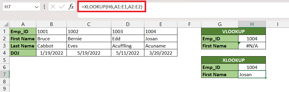
What’s the difference between vlookup and xlookup?
VLOOKUP is limited to looking up values to the right of the lookup column, whereas XLOOKUP allows you to retrieve information from any column, regardless of its position. Plus, XLOOKUP offers a search order option and the ability to provide a custom return value when a match isn’t found, eliminating VLOOKUP’s common issues with #N/A errors. This makes XLOOKUP a more flexible and user-friendly option in your Excel toolkit.
How do I VLOOKUP multiple criteria across different sheets?
To VLOOKUP with multiple criteria across different sheets, create a unique identifier in a helper column on each sheet by concatenating the criteria using the ‘&’ operator. Then, do a VLOOKUP using this unique identifier as your lookup value. Remember, your lookup range should encompass the helper columns you’ve created on the target sheet.
Conclusion
This completes our tutorial on how to use VLOOKUP to return values from multiple columns at once!
You can learn more about VLOOKUP basics, VLOOKUP with multiple criteria, and VLOOKUP in multiple sheets.

John Michaloudis is a former accountant and finance analyst at General Electric, a Microsoft MVP since 2020, an Amazon #1 bestselling author of 4 Microsoft Excel books and teacher of Microsoft Excel & Office over at his flagship MyExcelOnline Academy Online Course.


