The Ultimate Guide to HLOOKUP Function in Excel

HLOOKUP, or Horizontal Lookup, is a function in Microsoft Excel used to search for a value in the top row of a table or range and return a value in the same column from a specified row. It’s particularly useful when dealing with data organized horizontally, allowing for efficient data retrieval based on a reference value.

By specifying the lookup value, the table array, the row index number, and an optional range lookup parameter, HLOOKUP function streamlines the process of finding and extracting information within large datasets.

Key Takeaways:

• HLOOKUP is designed for searching a specific value across the top row of a table or range and returning a corresponding value from a specified row, making it ideal for horizontally organized data.
• Using the “FALSE” argument ensures exact matches, providing accurate data retrieval without the need to manually search through rows, thus enhancing efficiency in data analysis.
• Common pitfalls include inaccurate lookup values, not using “FALSE” for exact matches, and confusion between rows and columns. Avoiding these mistakes ensures smooth and reliable function performance.
• HLOOKUP can leverage wildcards for partial text matches, allowing for flexible and dynamic data searches even when exact details are uncertain.
• While HLOOKUP searches horizontally, VLOOKUP searches vertically. Understanding the orientation of your data helps in choosing the right function to streamline your data processing tasks effectively.

 

Introduction to HLOOKUP Mastery

Understanding the Essentials of HLOOKUP

Excel not only crunches numbers—it connects them in meaningful ways. Mastering the HLOOKUP function empowers you to link data horizontally, and this command becomes indispensable in your analytical toolkit. At its core, HLOOKUP is all about searching for a specific value across the top row of a table or range and returning a value in the same column from a row you specify.

Imagine a spreadsheet as a grid; HLOOKUP takes a horizontal path to find what you need. Eager to start? Imagine a simplistic table with sales figures and their corresponding regions —your goal is to extract a figure quickly.

With an HLOOKUP function, that once-daunting task becomes a single, swift formula away.

Why Excel Gurus Embrace HLOOKUP

Excel wizards have a knack for choosing the right tool for the job, and HLOOKUP is often their go-to when dealing with data spread across rows. Why? For starters, it’s incredibly efficient for pulling out specific information like price lists, timelines, or even student grades aligned in rows.

Plus, they love its flexibility—HLOOKUP easily adapts to various layouts and is excellent for crafting clean, readable reports. And when speed matters, they count on HLOOKUP’s direct approach to fetch data without the need to scroll through row upon row.

Speed, accuracy, and efficiency—HLOOKUP opens up possibilities for dynamic data interaction in ways that other functions simply can’t match.

 

Harnessing the Power of Horizontal Lookup

Example 1: Basic HLOOKUP Usage

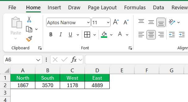
Ready to roll up your sleeves and dive into HLOOKUP? Let’s start simple. Picture a table displaying different regions and their sales targets for the year, all aligned horizontally. Your mission is to find the sales target for the North region.

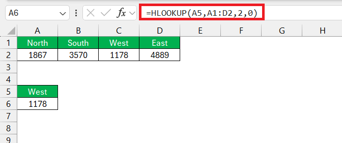
Here’s the magic formula you’d use: =HLOOKUP("North", A1:D1, 2, FALSE). In English, this translates to “Hey Excel, look for the word ‘West’ in the first row of the range A1 to D1 and give me the value from the second row of the column where you find ‘West’, and make sure it’s an exact match.” When you press Enter, like a faithful hound, Excel fetches the precise number you’re after.

This fundamental example shows how HLOOKUP streamlines data retrieval into a stress-free task.

Example 2: Dynamic HLOOKUP with Wildcards

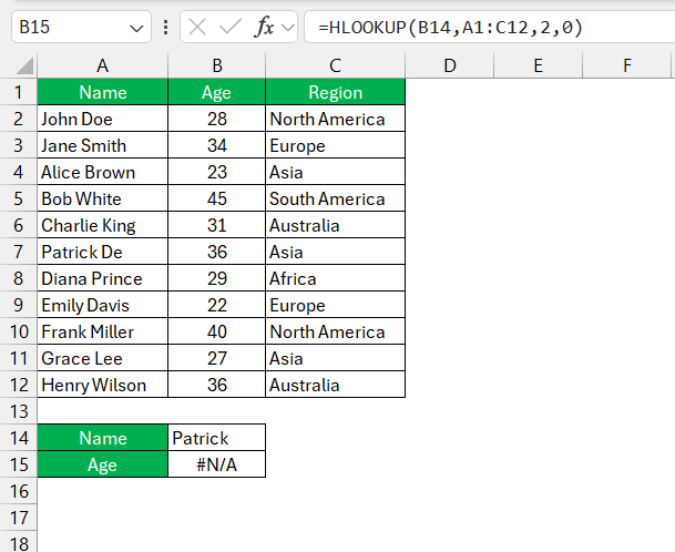
Now that you’ve grasped the basics, here’s how you turn the dial up a notch. When precision eludes you (like if you’re not 100% certain of a name or term), you can enlist wildcards in your search with HLOOKUP. Let’s say you have an employee roster, and you need to find details for a colleague whose name begins with “Pat”.

Using wildcards, your formula would be =HLOOKUP("Pat*", A1:Z2, 2, FALSE).

This tells Excel to play detective and look for any name in the first row starting with “Pat”, regardless of what follows. Asterisks act as placeholders for any string of characters, while question marks substitute for single characters, ideal when you’re unsure of a spelling or want to match any character in a specific position.

By harnessing wildcards, HLOOKUP transcends from a mere lookup tool to a powerful ally in data mining, even when the details are fuzzy.

 

Overcoming Common HLOOKUP Pitfalls

Top Mistakes and How to Avoid Them

Even Excel champions can trip over HLOOKUP’s quirks, so here’s your cheat sheet to avoid common missteps:

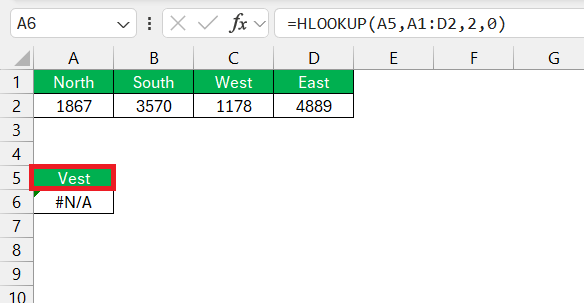
1. Inaccurate Lookup Value: If your lookup value isn’t a mirror image of the data, the function will return an error. To dodge this, double-check your value.

2. Not Using “FALSE” for Exact Match: Skipping the fourth argument in HLOOKUP might lead you down a path of approximate matches when you need precision. Always use “FALSE” or “0” to ensure an exact match.

3. Confusing Rows with Columns: Expecting HLOOKUP to search vertically instead of horizontally is like expecting a cat to bark. Remember, HLOOKUP is all about the horizon.

4. Moving Table Data: Your HLOOKUP function is tied to your data range. If that range changes but your function does not, expect errors to pop up. If your table is dynamic, consider using Excel’s Table feature or named ranges.

5. Overlooking the Need to Update the Row Index Number: When you add or delete rows within the lookup range, update the row index number accordingly or your HLOOKUP will be fetching data from the wrong row.

Steer clear of these pitfalls, and your journey with HLOOKUP will be smooth sailing.

 

FAQs on the HLOOKUP Function

Q1 :How do you use hlookup in Excel?

In Excel, you can use HLOOKUP to find a value in the top row of a table or range and return a value from the same column. Simply enter =HLOOKUP(lookup_value, table_array, row_index_num, [range_lookup]) into a cell.

Replace lookup_value with what you’re searching for; input table_array for the area containing the data; row_index_num specifies from which row to return the value; and [range_lookup] is optional to define the exact or approximate match.

Q2: What if the HLOOKUP can’t find the Lookup value?

If HLOOKUP can’t find the lookup value, it returns an #N/A error. To handle this, wrap your HLOOKUP in an IFERROR or IFNA function, such as =IFERROR(HLOOKUP(lookup_value, table_array, row_index_num, FALSE), "Custom Error"), which will display “Custom Error” (or any message you choose) instead of the #N/A.

Q3: Can HLOOKUP search for values in rows other than the first row?

No, HLOOKUP is designed to search only in the first row of the table_array. To look up values in other rows, you would need to reorganize your data accordingly or use a different function, such as INDEX-MATCH, which offers flexibility in choosing the row to search for the lookup value.

Q4: What is the difference between VLOOKUP and HLOOKUP?

VLOOKUP and HLOOKUP are similar in functionality, but they search in different orientations. VLOOKUP searches for a value in a specified column and returns a value from the same row in another column, while HLOOKUP searches for a value in a specified row and returns a value from the same column in another row. Use VLOOKUP for vertical searches and HLOOKUP for horizontal searches.

Q5: Can HLOOKUP handle arrays and wildcards effectively?

Yes, HLOOKUP can work with arrays and handle wildcards effectively. It’s great for searching partial text matches within the top row of a table array. Use the asterisk (*) to represent any sequence of characters or the question mark (?) for any single character. Ensure to set the range_lookup argument to FALSE for exact matching with wildcards.