7 Easy Steps to Master INDEX MATCH with Multiple Criteria

Key Takeaways

• The INDEX MATCH formula with multiple criteria in Excel allows for a precise data search and retrieval, even when there are no unique lookup values, a feature not commonly found in other lookup formulas without adding additional helper columns.
• To handle multiple criteria effectively, concatenate criteria using the ampersand (&) sign, which eliminates the need for complex array formulas, streamlining the process into a more straightforward and error-resistant approach.
• Applying the INDEX MATCH with multiple criteria involves three main steps: starting with a basic INDEX MATCH structure, altering the MATCH lookup value to 1, and carefully composing the criteria with concatenated lookup values and arrays to match the specific data needs.

Formula Syntax

The general syntax for the Index Match function is –

=INDEX(array, MATCH(lookup_value, lookup_array, [match_type])

What it means:
=INDEX(return the value/text, MATCH(from the row position of this value/text))

It can also be used when the result column is on the left side of the array. This is not possible when you are using VLOOKUP or HLOOKUP functions.

Index Match can be used if you have multiple criteria that you need to check in order to get the resultant value. Let’s understand this in a detailed step-by-step tutorial below.

• Array Function
• Non-Array Function

 

Download the Excel workbook to practice this tutorial on how to use Index Match with multiple criteria and follow along:

 

Array Function

The general syntax for Index Match with multiple criteria is –

=INDEX(return_range,MATCH(1,(criteria1=range1)*(criteria2=range2)*(criteria3=range3),0))

• return_range – It is the range that contains the lookup value
• criteria1, criteria2, and criteria3 are the conditions that need to be met
• range1, range2, and range3 are ranges on which the corresponding criteria should be tested

This is an array formula so you must hit Ctrl + Shift +Enter for the formula to work!

 

The test array will return TRUE or FALSE as a result where TRUE indicates that the condition has been met and similarly FALSE means the condition has not been met. The multiplication operator will convert the TRUE and FALSE to 1s and 0s. The row matching both criteria will return the value as “1”.

So, when a criteria is met, the resultant block in the formula would get converted to 1. As we are multiplying all the results,  the row matching both the criteria will return the value as “1”. Even if 1 criteria is not met, the entire value will become 0 or FALSE.

The MATCH function will return the position of the value 1 and the Index function will provide us with the resultant value.

Let’s look at an example to help us understand better.

 

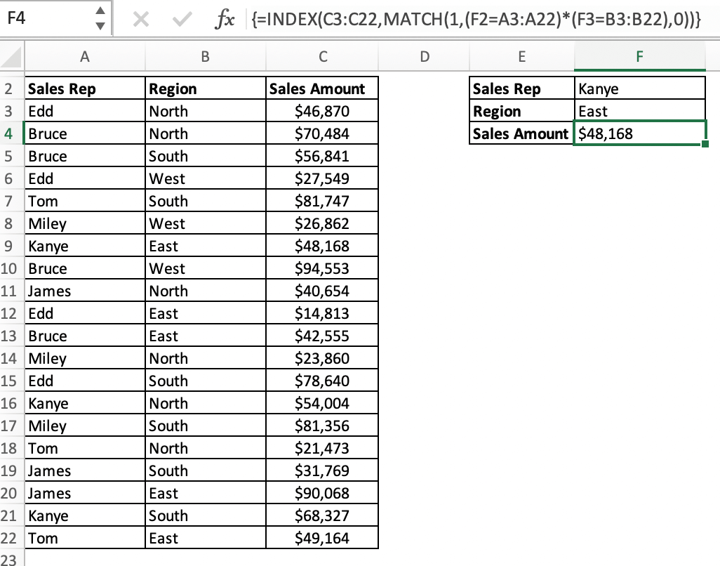
In the example below, we want to match two criteria – Sales Representative and Region and use Index Match to provide the corresponding sales amount matching the criteria.

STEP 1: Enter the INDEX formula

=INDEX(

STEP 2: Enter the first argument of the INDEX formula – array. This is the array that contains the lookup value. Here, it is the column containing the sales amount.

=INDEX(C3:C22,

STEP 3: Enter the MATCH function

=INDEX(C3:C22,MATCH(

STEP 4: Enter the first argument of the MATCH function – lookup_value. Here, it is the value “1”.

=INDEX(C3:C22,MATCH(1,

STEP 5: For the second argument i.e. lookup_array -we enter our criteria. Here we are searching on the basis of two criteria – Sales Representative name and Region. So you need to enter the two tests –

• If the Sales Representative (A3:A22) is Kanye (F2)
• If the Region (B3:B22) is East (F3)

You need to multiply the values of these two tests.

=INDEX(C3:C22,MATCH(1,(F2=A3:A22)*(F3=B3:B22)

STEP 6: Enter 0 for an exact match.

The match_type argument specifies how Excel matches lookup_value with values in lookup_array.

• The default value for this argument is 1. MATCH finds the largest value that is less than or equal to lookup_value.
• If we want an exact match, we enter 0.
• The last option here is -1. MATCH finds the smallest value that is greater than or equal tolookup_value)

=INDEX(C3:C22,MATCH(1,(F2=A3:A22)*(F3=B3:B22),0))

STEP 7: Press Ctrl + Shift + Enter.

This is crucial for our array function to work.

{=INDEX(C3:C22,MATCH(1,(F2=A3:A22)*(F3=B3:B22),0))}

 

You can highlight the test array and press F9 to see that the function gets converted to TRUE and FALSE –

=INDEX(C3:C22,MATCH(1,({FALSE;FALSE;FALSE;FALSE;FALSE;FALSE;TRUE;FALSE;FALSE;FALSE;FALSE;FALSE;FALSE;TRUE;FALSE;FALSE;FALSE;FALSE;TRUE;FALSE})*({FALSE;FALSE;FALSE;FALSE;FALSE;FALSE;TRUE;FALSE;FALSE;TRUE;TRUE;FALSE;FALSE;FALSE;FALSE;FALSE;FALSE;TRUE;FALSE;TRUE}),0))

Once multiplied, the expression gets converted to 0s and 1s.As we were multiplying, only the row that had fulfilled both criteria got converted into 1 or TRUE-
=INDEX(C3:C22,MATCH(1,{0;0;0;0;0;0;1;0;0;0;0;0;0;0;0;0;0;0;0;0},0))

The match function will now provide the relative position of the row for which all the criteria are TRUE. In this example, it is the 7th position.

=INDEX(C3:C22,7)

The Index function will provide the 7th value from the range C3:C22. The resultant value will be –

=48168

 

Non-Array Function

For an array function to work, you need to make sure that you press Ctrl + Shift + Enter together. If you simply press enter, the formula will break. An array function can be a little tricky to use, so you can add another INDEX function to catch the array function. To do this, INDEX is set up with one column and zero rows.

The three arguments of the 2nd Index function will be –

• array – the 2 tests i.e., If the Sales Representative (A3:A22) is Kanye (F2) and if the Region (B3:B22) is East (F3)
  (F2=A3:A22)*(F3=B3:B22)
• row_number – It will be 0, this will cause the index function to return the column specified.
• col_number – It will be 1, as the resultant array will only be 1 column.

=INDEX((F2=A3:A22)*(F3=B3:B22),0,1)

The final formula will be –

=INDEX(C3:C22,MATCH(1,=INDEX((F2=A3:A22)*(F3=B3:B22),0,1),0))

Even though this new formula is more complicated, it will surely work without having to press Ctrl + Shift + Enter. This formula can come in handy as people can forget to press Ctrl + Shift + Enter, causing our earlier formula to break.

Streamlining Your Workflow

Tips for Maintaining Readable and Efficient Formulas

Keeping your formulas readable and efficient isn’t just for your benefit; it’s for anyone who may inherit your Excel wizardry in the future. Start by breaking complex formulas into smaller, bite-sized pieces. If your formula spans several lines, chances are it could be simplified – making both troubleshoots and understanding as breezy as a walk in the park.

Adopt the habit of commenting directly within your formulas. Using the N() function, you can add text notes that won’t affect the computation but will offer valuable insights to anyone examining your work: =INDEX(D2:D13, MATCH(1, (G1=A2:A13) * (G2=B2:B13), 0)) + N("Matches criteria from G1 with A2:A13 and G2 with B2:B13")

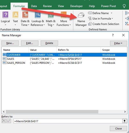
Also, clarity is the soul of usability. Break free from the shackles of cell references like $A$1, which can turn any formula into a maze of alphanumeric chaos. Instead, named ranges can be your beacon of light, guiding you through with meaningful terms related to your data’s content.

Keep in mind that simplicity triumphs complexity. By keeping your formulas lean, you aren’t just saving time – you’re crafting a spreadsheet that’s more accessible, more understandable, and ultimately, more useful.

Utilizing Named Ranges and Tables for Clarity

Embracing named ranges and tables in Excel might just be the hack you need for a seamless, comprehensible spreadsheet experience. Say goodbye to cryptic cell references like ‘B2:X2’ that leave you scratching your head. Instead, introduce yourself to the elegance of named ranges, giving your cell clusters meaningful names that convey their purpose with a glance.

Consider this: instead of the austere ‘$A$2:$A$13’, how about ‘ProductPrices’ or ‘ClientList’? With such clarity, your formulas become self-explanatory narratives, the kind that would make Excel proud. To create a named range, simply select the cells you want to name, go to the Name Box next to the formula bar, type your chosen term, and press Enter – it’s that simple.

Tables, on the other hand, aren’t just for their aesthetic appeal; they’re power tools disguised as grids. By converting your data range into a Table (by pressing Ctrl+T), you unlock table-friendly features like structured references. These automatically adjust when you add or remove data, making your formulas resilient to change.

Picture this: instead of updating a formula to account for new entries, your table-based formula adapts effortlessly, automatically. That’s less time tweaking formulas and more time for the important stuff.

With named ranges and tables working in harmony, complexity takes a back seat, allowing clarity to take the wheel.

Integrating INDEX MATCH with Other Excel Features

Powering Pivot Tables with INDEX MATCH Lookups

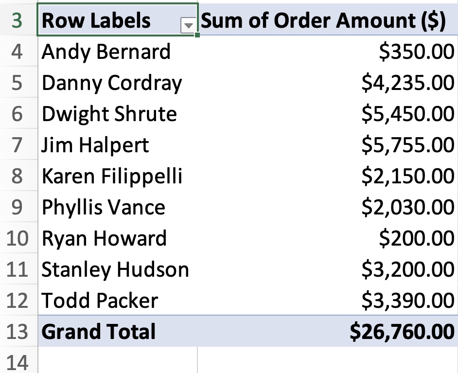
Pivot Tables are Excel’s built-in powerhouse for data summarization—a virtual Swiss Army knife for anyone looking to slice and dice figures. Combine the might of Pivot Tables with the finesse of INDEX MATCH lookups, and you unlock new realms of data manipulation.

Imagine seamlessly integrating a Pivot Table with data pulled through INDEX MATCH lookups. You can create calculated columns in your source data that dynamically retrieve and align relevant information with your Pivot Table’s summarized view. The result? A detail-rich, high-level analysis that unveils the stories behind the numbers.

Here’s an enticing thought: Your Pivot Table can automatically reflect changes in the data fetched by INDEX MATCH, ensuring that your summaries are always up-to-date. Simply refresh the Pivot Table whenever new data arrives, and watch as it recalibrates, as if by magic, filled with fresh insights.

With INDEX MATCH empowered Pivot Tables, tagging every twist and turn of your data becomes a relaxed stroll through a park, rather than a hurdle race.

Dynamic Charts Using INDEX MATCH with Multiple Criteria

Creating dynamic charts in Excel typically calls for dynamic ranges—the kind that can expand or contract with your dataset. Throw INDEX MATCH into the mix with multiple criteria, and you’ve got a recipe for charts that virtually update themselves as your data grows or changes.

You can set up a system where INDEX MATCH determines the range of data that feeds into a chart, allowing you to control what information is displayed based on certain criteria. Imagine a chart that adjusts to display sales data for different regions, products, or timeframes based on your selection—it’s like having a dashboard that bends to your will.

To make this magic happen, you often need to get comfortable with combining INDEX MATCH functions within named ranges – these named ranges can then be linked to your chart. As your data shifts, so too does the scope of the named ranges, ensuring your chart visuals are always relevant and to the point.

Let them marvel at how your charts breathe with the life of your data, evolving with each new entry or adjustment.

FAQ: Conquering Complex Data Searches

How does INDEX MATCH handle duplicate values with multiple criteria?

When you encounter clones in your data with INDEX MATCH handling multiple criteria, the process typically returns the first match it stumbles upon. It doesn’t have a built-in duplicate radar, so to speak. That means if you’re searching for a combo criteria that happens to pop up more than once, INDEX MATCH will unveil the first instance, blissfully unaware of its twin further down the list. If catching duplicates is your game, consider additional strategies like adding a helper column or refining your criteria to make your matches as unique as a snowflake.

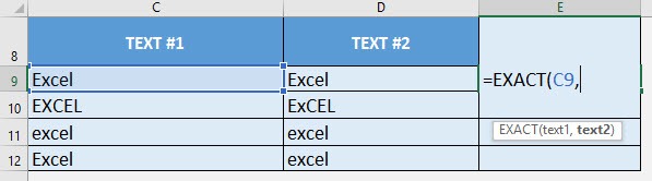
Is it possible to perform a case-sensitive lookup with INDEX MATCH?

Yes, it’s within your grasp to conduct a case-sensitive search with INDEX MATCH by bringing EXACT into the picture. Ordinarily, this tag-team isn’t picky about uppercase or lowercase letters, but EXACT changes the game. It’s like a detective that distinguishes between ‘Apple’ and ‘apple’, ensuring precision in your data quest. Remember though, you’ll be delving into array formula territory, which means sealing the deal with the special handshake of Ctrl+Shift+Enter in Excel versions prior to Excel 365.

What are some best practices for documenting INDEX MATCH formulas in Excel?

To make your INDEX MATCH formulas in Excel as transparent as a freshly cleaned windowpane, think like a librarian—organization is the key. Sprinkle your formulas with comments using Excel’s N function. It’s like leaving breadcrumbs for anyone following your trail through the spreadsheet. Create a legend or a notes section that maps out what each formula is doing, or perhaps a separate ‘Documentation’ sheet if you’re feeling extra meticulous. Embrace named ranges for a clearer narrative and less of that ‘$A$1’ code-speak.

Conclusion

You can either use an array function and make sure to press Ctrl + Shift + Enter for the function to work. Or, you could simply add another Index function if you wish to use a non-array function.

Click here to learn more about Index Match and other lookup functions in Excel.