Table of Contents
Pivot Charts & Slicers
In a previous post I showed you how to Insert a Pivot Chart. Now we will take this concept once step further and insert a Slicer. The cool thing about this is that the Slicer will control both the Pivot Table and the Pivot Chart.
See how you can start creating some awesome interactive analytical reports in just a couple of steps.
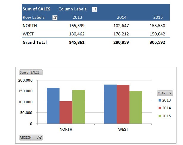
Here we have our Pivot Table and Pivot Chart ready:
STEP 1: Click in your Pivot Table and go to Options > Insert Slicer
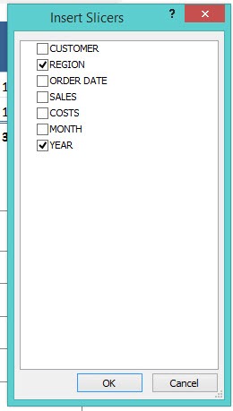
STEP 2: Select Region and Year. Click OK
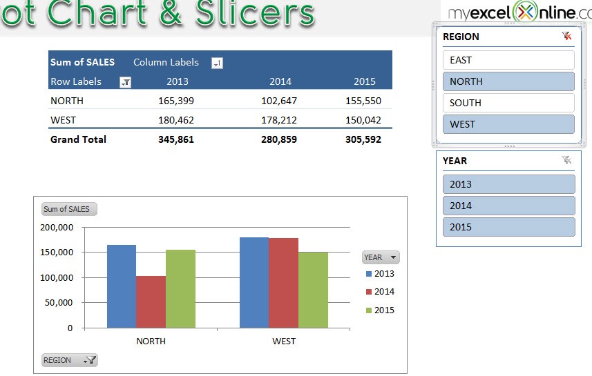
You now have your Slicer and you can play around with it! It will affect both the Pivot Table and Pivot Chart!
John Michaloudis is a former accountant and finance analyst at General Electric, a Microsoft MVP since 2020, an Amazon #1 bestselling author of 4 Microsoft Excel books and teacher of Microsoft Excel & Office over at his flagship MyExcelOnline Academy Online Course.


