Excel Recovery Rate: Step by Step Formula Guide

Introduction to Recovery Rate

What is the Recovery Rate?

When navigating the challenging waters of finance, the “recovery rate” serves as a beacon, guiding lenders and businesses through the fog of default and bankruptcy. Simply put, this percentage reflects the portion of defaulted debt that can potentially wiggle its way back into the lender’s pocket. They illuminate the endgame—how much of their outlaid capital might return home after a detour with default.

Why is it Important? Understanding the recovery rate transcends mere curiosity—it’s a cornerstone of credit risk management. Lenders, clinging to this number, can estimate the eventual recoupment from their loans gone awry. For a lender, a high recovery rate is the light at the end of the tunnel, hinting at fewer losses and greater financial resilience.

Understanding the Basics of Recovery Rates

Defining Recovery Rate in Finance

In the meticulous world of finance, defining the recovery rate is pivotal. It stands as a quantitative measure expressing the proportion of a defaulted loan that is likely to be recouped. Essentially, it’s a lens providing clarity on what percentage of the lent funds could be salvaged in the unfortunate event that a borrower cannot fulfill their debt obligations. Whether one is dealing with corporate bonds, individual loans, or credit facilities, the recovery rate is a crucial factor in painting a realistic picture of potential financial outcomes.

The Formula and How It Works Let’s get numerical. Calculating the recovery rate is akin to solving a puzzle—the key is knowing exactly where each piece fits. The formula itself is straightforward:

Recovery Rate = Total Recovered Value/Original Loan Amount * 100

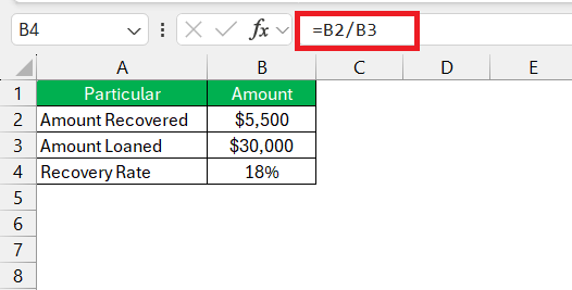
This equation is your tool for transforming raw data into actionable financial insights. In practice, you’d take the total amount recovered from a defaulted loan and divide it by the loan’s original value. Multiply by 100 to get a percentage, and voilà—you have your recovery rate. This figure isn’t just decorative; it’s instrumental in figuring out the Loss Given Default (LGD) with a simple adjustment:

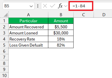
Loss Given Default (LGD) = 1 – Recovery Rate

By flipping the recovery rate on its head, you’re now peering into the world of potential losses. It sharpens your understanding of risk and cushions the blow of defaults by setting realistic loss expectations.

The Formula and How It Works

To navigate financial risks like a seasoned explorer, you must grasp the recovery rate’s formula. It’s relatively simple and can be a lifesaver in a sea of default uncertainties. Here’s the lifesaver in its numerical form:

Recovery Rate = Total Recovered Value/Original Loan Amount * 100

This formula unfurls the mystery behind a loan’s potential comeback once it hits a snag. By dividing the amount you’ve managed to salvage post-default by the original value of the loan and catapulting it into percentage form, you get the recovery rate. This isn’t just a number—it’s the pulse of your investment, revealing how strong or feeble it stands after a blow.

Excel, with its convenient computational magic, lets you translate this formula into a dynamic beacon, illuminating the pathway to smarter, data-driven decisions. Understanding this formula is akin to knowing your ship’s coordinates at sea; it can make the difference between a voyage to treasure or a drift toward loss.

Step-by-Step Guide to Calculating Recovery Rate in Excel

Setting Up Your Data Table

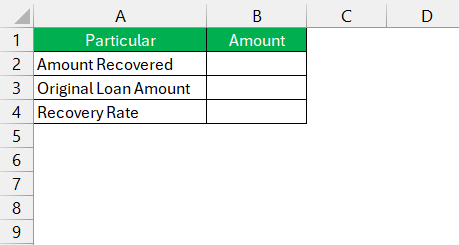
Before setting sail on the vast ocean of data, you need to arrange your navigational charts—that is, set up your Excel data table meticulously. Here’s a tip to avoid your data becoming a Bermuda Triangle:

STEP 1: Label your columns appropriately; something like “Original Loan Amount,” “Amount Recovered,” and “Recovery Rate” will work wonderfully.

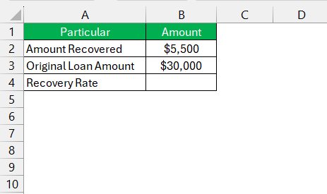
STEP 2: Fill in the “Original Loan Amount” and “Amount Recovered” columns with the respective figures for each defaulted loan.

The “Recovery Rate” column is where the magic happens, but it’ll remain an empty treasure chest for now, awaiting the golden formula.

This preparation ensures that when you apply the recovery rate formula, Excel will be ready to calculate with the precision of a seasoned navigator charting a course through calm seas.

Applying the Recovery Rate Formulas

Now that your data table is set up with the rigor of a ship’s logbook, you’re ready to apply the recovery rate formulas with the precision of a seasoned captain. Here’s how to plot the course:

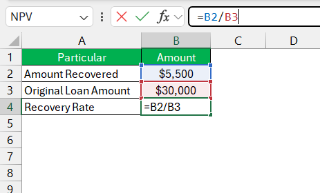
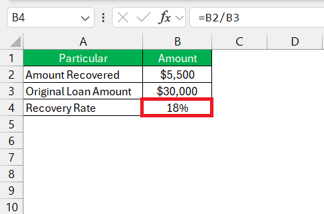
STEP 1: In the “Recovery Rate” column cell, where your journey starts, enter the Excel formula: =B2/B3*100 (assuming B2 is the “Amount Recovered” and B3 is the “Original Loan Amount”).

STEP 2: Strike the “Enter” key like dropping an anchor and watch as Excel calculates the recovery rate for the first entry.

To replicate this formula for the entire column, click on the cell with the formula, find the small square at the bottom right corner (the fill handle), click, and drag it down to the last row of your data. This action auto-fills the formula, calculating the recovery rates for each row.

Seeing the calculated recovery rates populate the cells is akin to catching wind in your sails – with each figure, your understanding of your financial position grows clearer. Remember to format these cells as percentages for quick and easy reading as you navigate through your financial analysis.

Common Mistakes and Tips for Accurate Recovery Rate Calculation

Ensuring Correct Input Values

Before Excel can work its calculating magic, the sorcerer’s wand must be waved correctly—that is, ensuring your input values are accurate. Here’s how:

1. Verify each entry in the “Original Loan Amount” and “Amount Recovered” columns. Even the slightest miscalculation can lead your course astray, like a misguided compass.
2. Beware of common trip-ups like misread figures, swapped digits, or misplaced decimal points—errors that lurk in the shadows of data entry.

Maintaining vigilance here is the rigging on your mast; it keeps your calculations sailing true and prevents your conclusions from floundering in the deep. Remember, in the ocean of numbers, accuracy is the North Star.

Tips to Avoid Errors in Excel

Navigating the stormy seas of Excel without running aground on errors requires a keen eye and a steady hand. Here’s how you can keep your calculations on the straight and narrow:

1. Double-Check Your Formulas: A formula in Excel is like a compass; if it’s off by even a degree, you could end up leagues away from your destination. Always double-check your formulas for accuracy.
2. Use Excel’s Built-In Tools: Leverage features like ‘Formula Auditing’ to trace any errors and use ‘Data Validation‘ to avoid incorrect data entry from the get-go.
3. Maintain Spreadsheet Discipline: Keep your sea of cells organized with clear labels, consistent formatting, and strategic cell locking to avoid accidental overwriting.
4. Proofread with Fresh Eyes: Sometimes you need to step away from the helm and return with a fresh perspective to spot any mistakes.
5. Embrace Error Checking Functions: Incorporate error checking functions such as ISERROR or IFERROR to catch and manage errors smoothly, ensuring they don’t capsize your analysis.

Remember, vigilance and verification are your trusty crewmates in the voyage through Excel’s numeric ocean. With these guiding stars, you’ll skillfully steer clear of the common errors awaiting in hidden reefs.

Practical Applications of the Recovery Rate Formula

Analyzing Loan Defaults

When analyzing loan defaults, you’re decoding the narrative behind the numbers. Excel serves as your cipher, revealing the story of loans that have navigated into the choppy waters of non-payment. Here’s how to approach this analysis:

1. Use the recovery rate calculation to estimate the potential losses from defaults. By storing historical data on defaults and recoveries, you can anticipate future patterns.
2. Create a default analysis model in Excel to identify trends and risk factors. With conditional formatting, highlight loans with high-risk indicators that may be more prone to default.

Analyzing loan defaults with a tool as potent as Excel enables you to identify where the leaks are in your financial vessel and patch them up before setting sail again. It’s about turning data into decisions, and transforming what might seem like abstract numbers into tangible strategies for minimizing risk and maximizing recovery.

Assessing Company Health with Recovery Rates

Recovery rates are the financial pulse of a company, offering vital signs of its credit health and resilience. In evaluating a firm, they are a tool for forecasting the buoyancy of a company’s ability to weather the storm of defaults. Here’s how to assess company health:

1. Analyze the trends in a company’s recovery rates over time to spot indicators of improving or worsening credit health.
2. Compare these rates with industry benchmarks to gauge where the company stands in the rough seas of market competition.

Higher recovery rates often suggest a sturdy lifeboat, indicating that a company can reclaim a substantial portion of its issued credit, even when defaults occur. Conversely, lower rates might hint at potential leaks below the waterline, suggesting vulnerability.

By using recovery rates as a measure, you can forecast potential downturns and navigate towards more prosperous investment shores, ensuring that the company’s financial vessel is fit to sail through the turbulent waters of industry and economic challenges.

FAQs

What is the formula for recovery rate?

To calculate the recovery rate, the formula you’ll need is a straightforward beacon:

Recovery Rate = Total Recovered Value/Original Loan Amount * 100

Apply this formula to discover the percentage of recouped funds from the original amount lent or invested, lighting the way to comprehending your financial recovery journey.

What does recovery rate mean?

The recovery rate shines a light on the proportion of funds that lenders can retrieve after a borrower defaults. It’s a crucial metric that reflects the effectiveness of a company’s risk management tactics, helping to steer through the fog of credit losses.

Can I Compute Recovery Rate for Different Periods?

Yes, you can chart the recovery rate for different timeframes. Whether you’re keeping watch weekly, monthly, or annually, the formula remains your financial compass, guiding you through the temporal tides of debt recovery.

Where Can I Find More Examples of Recovery Rate Calculations?

You’ll find a treasure trove of recovery rate calculation examples in finance textbooks, online financial forums, and Excel-related websites. These sources can offer you a compass to navigate through various scenarios and datasets.

How to do rate of return on Excel?

Calculating the rate of return in Excel involves a simple process:

1. Input your investment cost and total returns into separate cells.
2. In a blank cell, craft the formula: = (Total Returns - Investment Cost) / Investment Cost.
3. Convert to percentage by clicking on the “%” icon.

This will unfurl the sails of your rate of return, guiding your investment decisions with precision.

John Michaloudis

Founder & Chief Inspirational Officer

at

MyExcelOnline.com

John Michaloudis is a former accountant and finance analyst at General Electric, a Microsoft MVP since 2020, an Amazon #1 bestselling author of 4 Microsoft Excel books and teacher of Microsoft Excel & Office over at his flagship MyExcelOnline Academy Online Course.