VLOOKUP Example: Vlookup with a Drop Down List

The VLOOKUP function in Excel can become interactive and more powerful when applying a Data Validation (drop down menu/list) as the Lookup_Value.  So as you change your selection from the drop-down list, the Excel VLOOKUP value also changes.

Key Takeaways:

• VLOOKUP can be effectively integrated with a drop-down list in Excel to retrieve specific data such as prices based on user selection.
• Creating a dynamic drop-down list in Excel requires the use of the Data Validation feature, which provides the user with a list of choices from a defined table. Post selection, other cell attributes like price or description can be automatically filled using VLOOKUP based on the named reference of the chosen item.

VLOOKUP Formula Syntax

What does it do?

Searches for a value in the first column of a table array and returns a value in the same row from another column (to the right) in the table array.

Formula breakdown:

=VLOOKUP(lookup_value, table_array, col_index_num, [range_lookup])

What it means:

=VLOOKUP(this value, in this list, and get me value in this column, Exact Match/FALSE/0])

Follow the step-by-step tutorial on Excel dependent drop down list Vlookup and download this Excel workbook to practice along

Vlookup with a Drop Down List Step-By-Step Guide

STEP 1: Go to Data > Data Validation. 

 

STEP 2: Select List in the Allow dropdown. 

For the Source, ensure that it has the 4 Stock List values selected. Click OK.

Your dropdown is ready.

 

STEP 3: We need to enter the Vlookup function in the Excel Vlookup example:

=VLOOKUP(

The Vlookup arguments:

lookup_value

What are we looking for?

Reference the cell that contains the text or value:

=VLOOKUP(G15,

table_array

From which list are we doing a lookup on?

Place in the cell range of the Stock List:

=VLOOKUP(G15, $B$14:$D$17,

col_index_num

From which column do we want to retrieve the value?

We want to retrieve the Price which is the SECOND column from our table array:

=VLOOKUP(G15, $B$14:$D$17, 2,

[range_lookup]

Do we want an exact match?

Place in FALSE to signify that we want an exact match:

=VLOOKUP(G15, $B$14:$D$17, 2, FALSE)

 

The price now dynamically changes based on your selection:

Advanced VLOOKUP Tricks

Handling #N/A Errors Gracefully

You may face #N/A error when using the VLOOKUP function in Excel. Excel returns this error when it is unable to find the search item in the list.

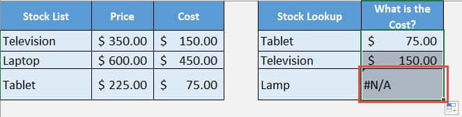
You can easily handle this error by using the IFERROR function. With this function, you can return a default value when VLOOKUP doesn’t find a match.

The formula looks like this:

=IFERROR(VLOOKUP(lookup_value, table_array, col_index_num, [range_lookup]), "Value not found")

Dynamical Drop Down Lists Using VLOOKUP

You can easily create dynamic drop down with a combination of data validation, INDIRECT, and VLOOKUP functions. These will be dependent drop down lists wherein when you select an item in the primary drop down list, the secondary list will change automatically.

If you make any change in the source data, the option in drop down will also be updated automatically.

 

Practical Examples

Inventory Management

You can easily manage your inventory with the combo of VLOOKUP and with drop-down list. Item names, stock levels, and prices can all be tracked using a well-organized table.  Once you select an item from the drop-down, VLOOKUP will pull data like stock price and quantity corresponding to the item you have selected. This will be useful for stock assessment and updating inventory records.

Below are the reasons why VLOOKUP with drop-down will be useful for you:

1. Instantly retrieve item information without manually searching through rows.
2. Reduce human error, since you are pulling data directly from a table.
3. Update inventory details swiftly, simply by changing the source table.

By integrating these Excel tricks, you’ll have a useful formula to keep your stock levels consistent and accurate, save time, and make inventory management a breeze.

Sales Reports and Performance Tracking Made Easy

When it comes to sales reports and performance tracking, VLOOKUP, combined with a drop down list, helps you create a dynamic reporting tool. You can easily track sales by product, region, or salesperson with a quick selection from a drop down list. VLOOKUP retrieves the relevant sales data, presenting you with up-to-the-minute reports. You can track performance trends over time, compare sales across different categories, or calculate commissions based on sales data—all without writing cumbersome formulas for each query.

Here’s why using VLOOKUP like this is a game-changer:

• Quickly adapt reports to display information that’s relevant to a specific audience or time period.
• Minimize the need for manual updates—when source data is refreshed, so are your report summaries.
• Information sharing among team members will be easy.

This approach ensures your sales reports are always ready for that last-minute meeting, with accurate data just a few clicks away.

FAQs

Why is VLOOKUP with drop-down returning #N/A error?

VLOOKUP may return #N/A error because of the following reasons:

• Please check if the value you are searching for is actually present in the data range.
• Match the format of the data with the drop down list.
• Make sure that the lookup range is correct

Once you resolve these issues, you will be able to use VLOOKUP smoothly.

After selecting a value from drop-down, can I use VLOOKUP to fill multiple columns?

Absolutely! You can use VLOOKUP to fill several columns based on a single item selected in drop-down. You can use the same formula but change the argument – column index to get data from different columns.