How to Flip Data in Columns and Rows in Excel

When working with data in Excel, you may find that it is not arranged in the format you need. Sometimes data is listed in columns when you need it in rows, or vice versa. This process is known as flipping data. In this article, you will learn different methods to flip data between columns and rows in Excel.

Key Takeaways:

• Flipping data means changing rows into columns or columns into rows.
• You can use Paste Special with Transpose to flip data.
• The TRANSPOSE function gives a linked output.
• INDEX can also help you flip data.
• SORTBY is useful for rearranging data, but not for flipping the layout.

 

Introduction to Flip Data in Excel

Flipping data means changing the orientation of the dataset. If the data is arranged vertically in columns, you can flip to display it in rows. In the same way, data arranged in rows can be flipped into columns.

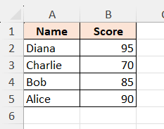
If the original data looks like this:

After flipping, the structure of the dataset changes from its original format.

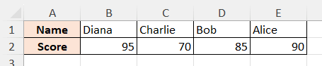
This is useful when you need to reorganise data for better readability.

 

How to Flip Data Horizontally

Using Excel Functions

Navigating through Excel’s treasure trove of functions can lead you to some pretty handy tools for data flipping. For a quick flip, they’ve got you covered with simple yet effective features. You don’t need to be a wizard; just use the ‘Sort’ button to reverse the order.

STEP 1: Select the data range.

STEP 2: Go to the Data > Sort > Sort Z to A.

STEP 3: Select the data range and copy it by pressing Ctrl+C.

STEP 4: Right-click on the target cell and select “Paste Special”.

STEP 5: Check the “Transpose” box and click “OK”.

RESULT:

TRANSPOSE Formula

The TRANSPOSE function can help you to flip data using a formula. It can convert vertical data into horizontal data, and horizontal data into vertical data. This helps you change the layout of your data without manually rearranging it.

This method is useful as the result updates automatically if the original data changes.

INDEX Function

You can use the INDEX function with the ROWS function to change data from rows to columns or columns to rows.

You can use this method to flip only part of the data or change the order in a specific way.

SORTBY Function

The SORTBY function allows you to reverse the order of your columns or tables with just a few clicks.

However, it does not flip rows into columns. It only rearranges the data in the same layout.

FAQs

Is there a way to flip the order of data in Excel?

You can use simple methods like SORT and PASTE SPECIAL or formulas like with TRANSPOSE or INDEX and ROWS to flip data vertically or horizontally.

How do you reverse the order of data?

To reverse data horizontally, follow the steps below:

• Create a helper row containing sequential numbers.
• Select your dataset along with this helper.
• Click ‘Data’ tab
• Select the Sort button
• Click on the ‘Options’ button
• Select ‘Sort left to right’

What is Excel transpose?

Excel Transpose is the feature that flips the layout of the data. It can change columns to rows, or rows to columns.

Does TRANSPOSE update automatically?

Yes, it updates when the original data changes.

Does SORTBY flip rows and columns?

No, it only sorts data, not changes the layout.