How To Fill Blank Cells in Pivot Table

Pivot Table is a great tool that can be used to summarize data in Excel. It lets you analyze more than 1 million rows of data with just a few mouse clicks. But the blank cells in the Pivot Table make it difficult for users to read the data. In this article, you will learn how to fill in blank cells in a Pivot Table with 0, N/A, or any custom text.

Key Takeaways

• Blank cells in a Pivot Table can make reports harder to read.
• Use PivotTable Options to replace blank cells with any value or text.
• You can display 0, N/A, or any custom text in empty cells.
• Changing empty cell values does not modify the source data.
• The new display applies to the entire Pivot Table instantly.

 

Watch it on YouTube and give it a thumbs-up!

Follow a step-by-step tutorial on How to fill blank cells in Pivot Table and download this Excel workbook to follow along:

Example 1:

Suppose you have this data set containing sales data as shown below:

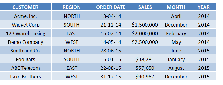
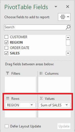
Using this data, a Pivot Table has been created by dropping region in the row field and sales in the values field.

 

The resultant Pivot Table is shown below.

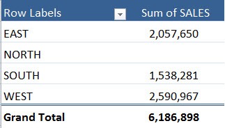
As you can see the pivot value for North Region is blank, let us change this! Follow the steps below to learn how to fill blank cells in Pivot Table with any custom text.

 

STEP 1: Click on any cell in the Pivot Table.

 

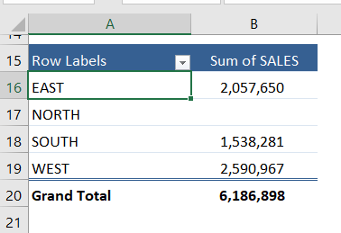
STEP 2: Go to PivotTable Analyze Tab > Options

 

STEP 3: In the PivotTable Options dialog box, set For empty cells show with your preferred value. Let’s say, you change pivot table empty cells to”0″.

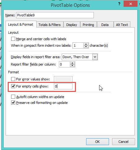
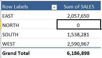
All of your blank values are now replaced!

 

You need to click in your Pivot Table > PivotTable Analyze > Options > Format > For empty cells show: enter a value or text in this box.

This is how you can replace pivot table blank cells with 0!

Let’s look at another example on how to fill blank cells in pivot table with a custom text.

 

Example 2:

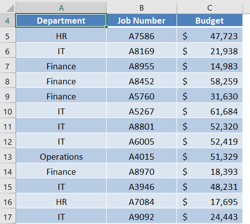
In this example, you can different departments and job numbers related to that department. A budget has been assigned to these items.

A Pivot Table is created with Job Number in Rows field, Department in Columns field and Budget in Values field. The result is shown below:

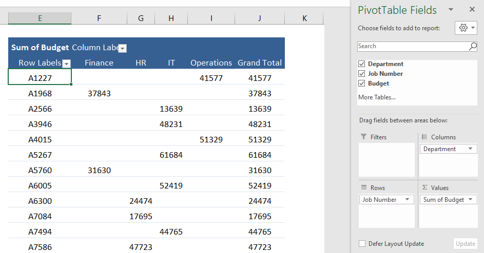
You might see there are blank cells in this Pivot Table. This is because there are no record for that particular row/column label.

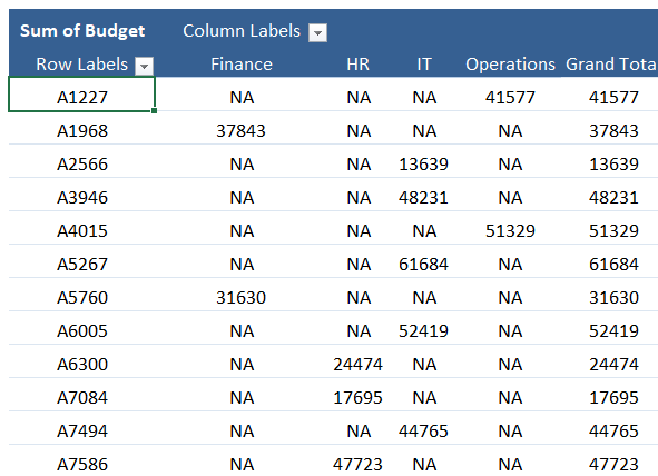
For example, there is no budget assigned for job number A1227 in Finance, IT and HR.

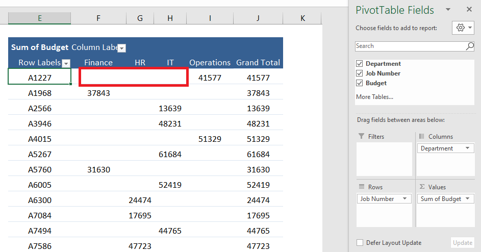
You can easily replace this blank cell with the text “NA”.

 

STEP 1: Right click on any cell in the Pivot Table.

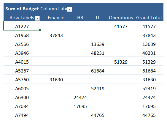
STEP 2: Select PivotTable Options from the list.

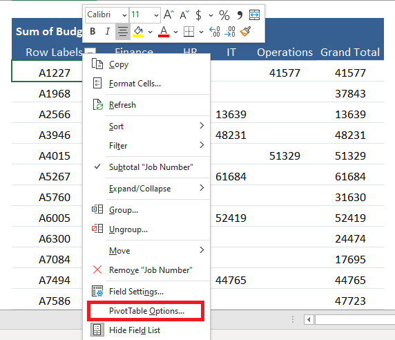
STEP 3: In the PivotTable options dialog box, enter NA in the field – For emply cells show:

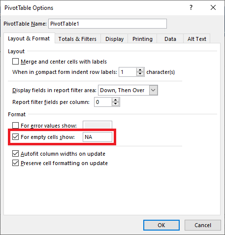
That’s it! All the blank cells will now show NA!

 

Tips and Tricks

• Use 0 for reports that contain numbers and calculations.
• Use N/A or another custom text when the value is not available.
• Refresh the Pivot Table after updating the source data.
• Keep your source data free of unnecessary blank cells for better reports.
• Use consistent replacement values throughout the workbook for easier analysis.

 

FAQs

1. Why do blank cells appear in a Pivot Table?

They appear when there is no data for a row and column combination.

2. How to replace blank cells with 0?

To replace blank cells with 0,

• Click anywhere inside the Pivot Table.
• Go to PivotTable Analyze > Options.
• Under Layout & Format, find For empty cells show.
• Enter 0 in the box.
• Click OK.

3. Can I display text instead of blank cells?

Yes. You can use text such as N/A or any custom value.

4. Will replacing blank cells change my source data?

No. It only changes how the Pivot Table displays empty cells.

5. Can I change the replacement value later?

Yes. Open PivotTable Options and enter a different value or text.