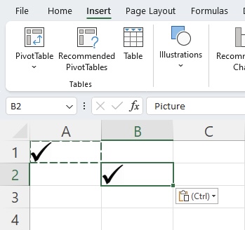
When creating spreadsheets, you might find yourself needing to insert check marks in Excel to indicate completion, approval, or other status markers. In this article, we’ll explore several methods for inserting check marks into your Excel worksheets.
Let’s look at each of these methods!
Download the Excel Workbook below to follow along the Inserting a Check Mark in Excel tutorial! –
download excel workbook CheckmarkinExcel.xlsx
Table of Contents
Copy and Paste
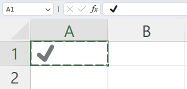
By far, the easiest way to insert a check mark in Excel is by simply Copying and Pasting this symbol: ✔
Highlight ✔ and right-click to copy or press CTRL + C.
Paste the checkmark in any cell in Excel by pressing Ctrl + V.
Note: This method is ideal for copying and pasting check marks in a few places manually. However, it is not practical for dealing with hundreds or thousands of cells, where using a formula (as explained later in this tutorial) is a better approach.
Using the Symbol Command
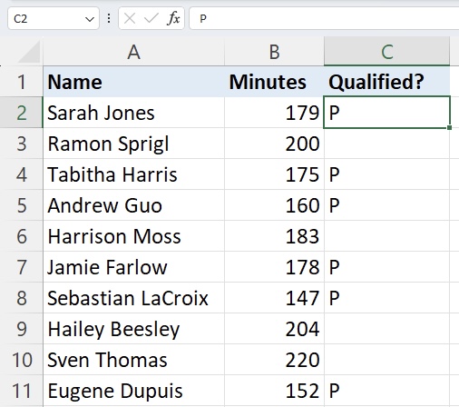
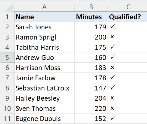
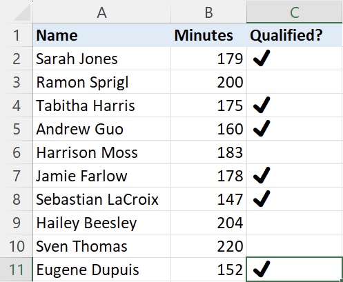
Let’s consider an example in the context of marathon race qualifiers. We will insert a checkmark in a cell to indicate whether an athlete has qualified for the race if their time is 180 minutes or below:
Enter the capital “P” or “Shift + P” on the cells where you want the check marks to be.
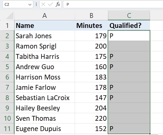
Highlight the range where you want to have the check marks.
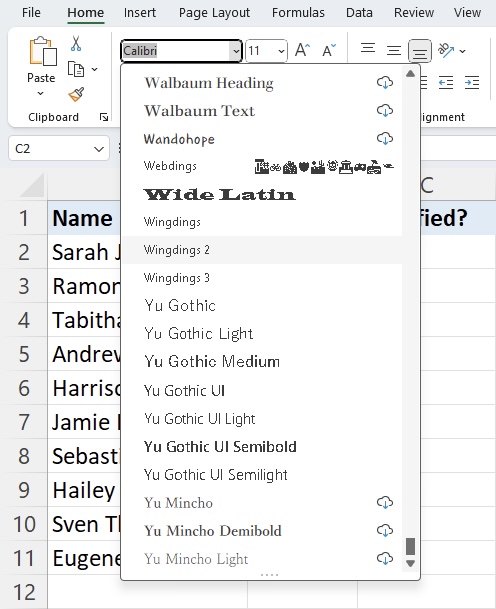
Go up to the Home ribbon and click the Fonts drop-down menu. Change the font from Calibri to Wingdings 2.
Additionally, if you wanted to mark down the failed qualifications with an “X”, you can enter the uppercase “O” in the cell.
As you can see, by changing the font from Calibri to Wingdings 2, the uppercase P has been changed to the check mark.
Check Marks with the CHAR Function
The CHAR function allows us to automate the process across a significant number of cells in an Excel spreadsheet.
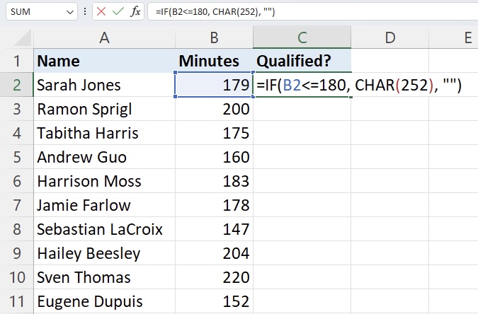
Assuming you want to insert a checkmark if the value in cell B2 is lesser than or equal to 180:
In cell C2 (or any other cell where you want the checkmark to appear), enter the following formula:
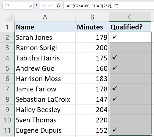
=IF(B2<=180, CHAR(252), “”)
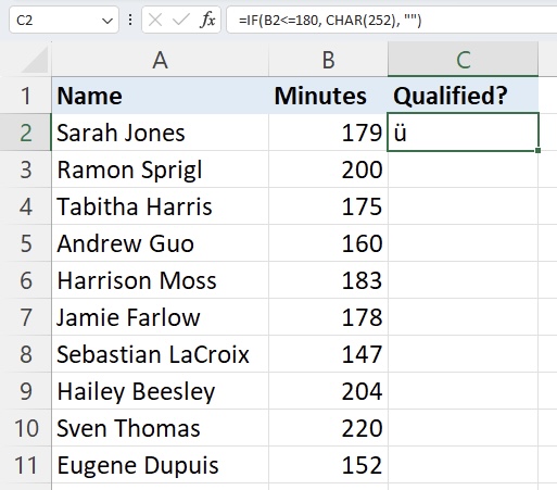
You may get a return with the symbol ü. That is perfectly fine. Apply the formula to the rest of the column by double-clicking the square on the bottom right-hand corner of cell C2.
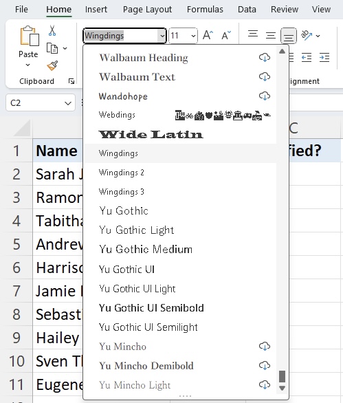
Highlight cell C2 to C11. Go up to the Home ribbon and change the font to Wingdings.
As you can see, the cell in column C will dynamically display a checkmark if the value in cell B2 is lesser than or equal to 180.
Insert a Checkbox
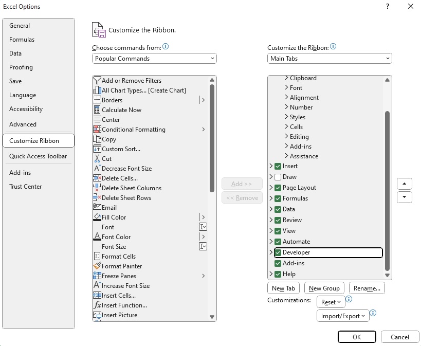
If you do not have the Developer tab on the Excel Ribbon, start by going to the File menu. Choose Options and click on Customize the Ribbon.
On the right side, make sure to check the box that says Developer.
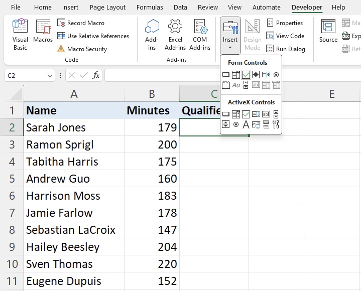
Click on the Developer tab, go to Insert, and select the checkbox.
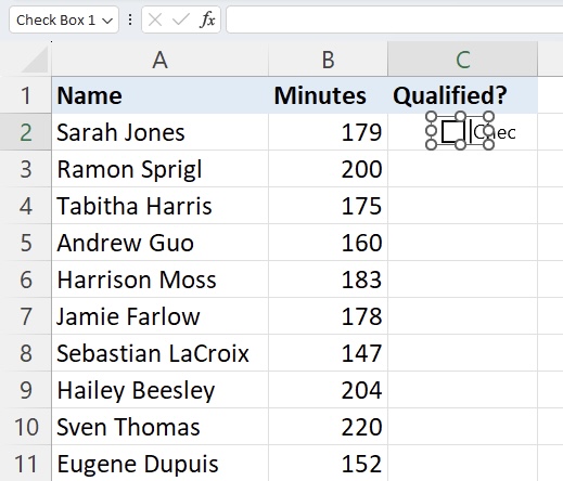
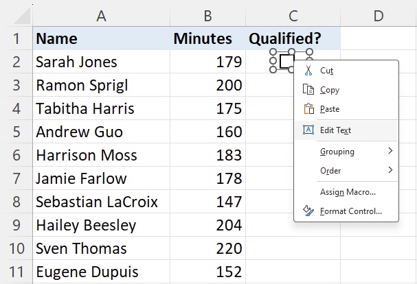
Click and drag where you want the check box to appear on the cell. You can edit the text or completely remove it by right-clicking and selecting Edit Text.
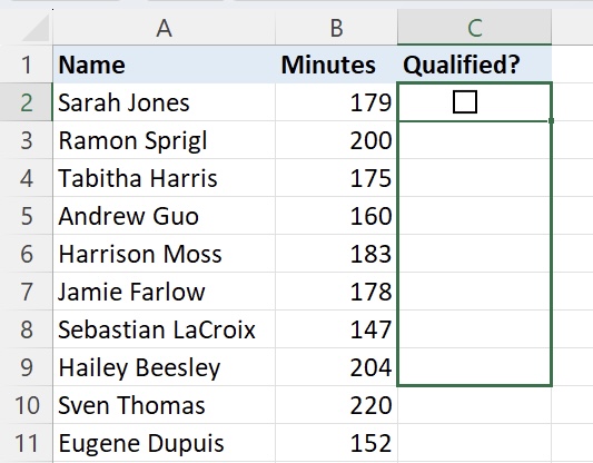
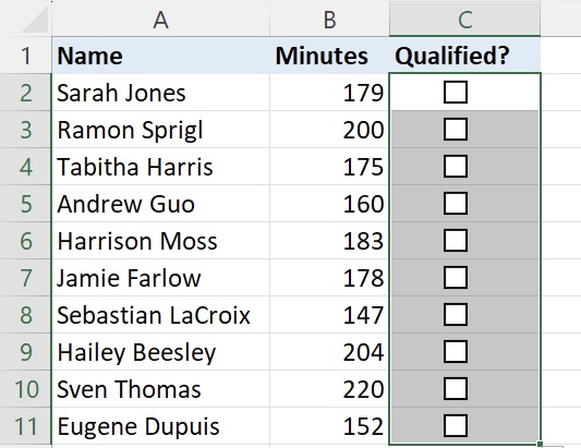
Locate the small square on the bottom right-hand corner of the cell and drag down to apply the check box to the rest of the cells.
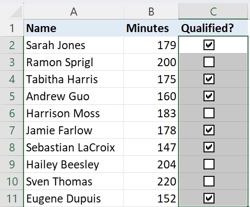
Now you can freely check or uncheck the box depending on whether the athletes qualification time.
There are many other methods for inserting checkboxes in Excel!
Check Mark in Excel with AutoCorrect
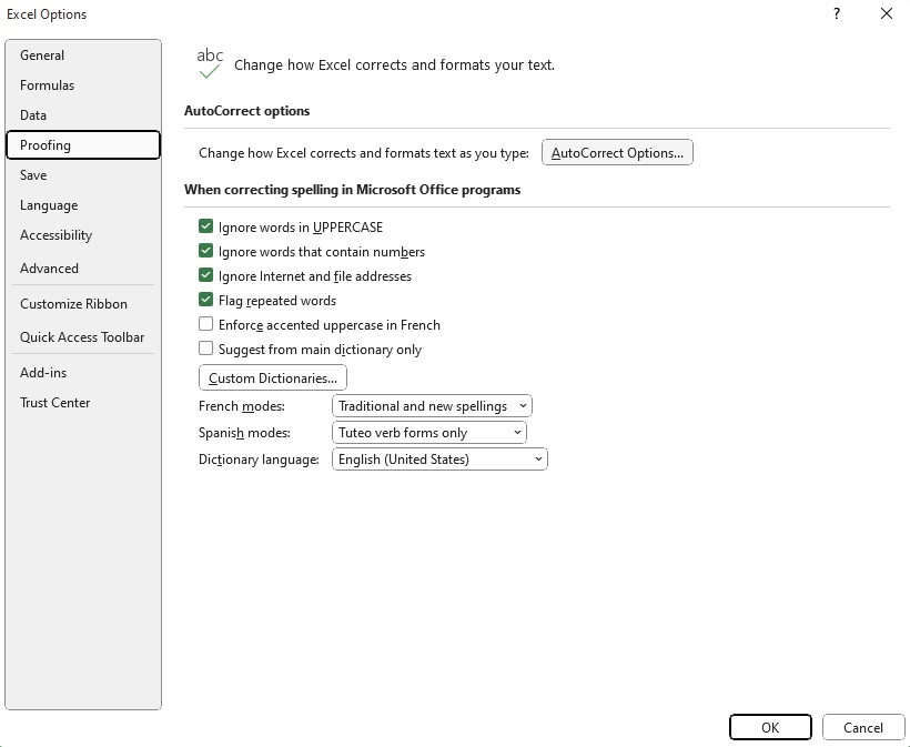
AutoCorrect has many handy uses in Excel. But did you know you could replace a text with a check mark? Go to the File tab, select Options, and choose Proofing.
Click on AutoCorrect Options.
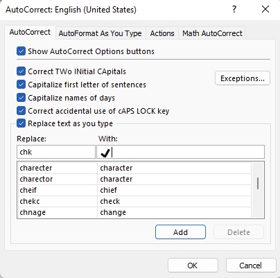
In the Replace box, type the shortcut “chk” and in the “With” box, enter the check mark symbol.
Click Add and then OK.
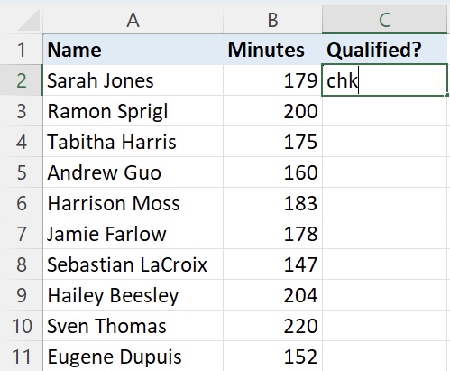
Enter chk in cell C2.
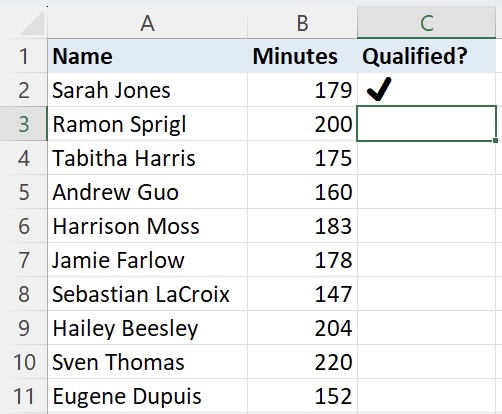
As you can see, Excel will AutoCorrect chk with the ✔️ mark.
Conditional Formatting
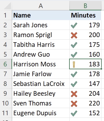
Let’s say you want to insert a checkmark in column B when the value in the corresponding cell in column B is lesser than or equal to 180. This can be achieved with the power of Microsoft’s Conditional Formatting.
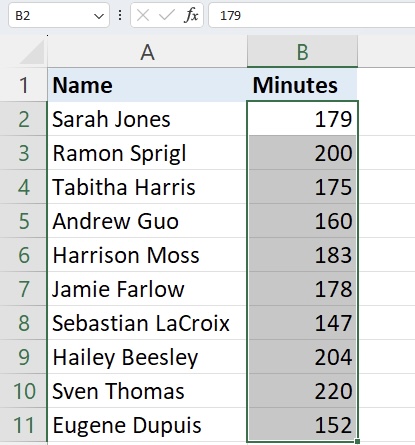
Highlight the entire column or the range where you want the conditional formatting to be applied.
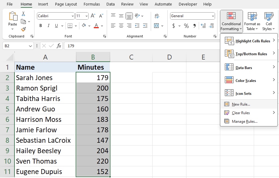
Go to the Home tab on the Excel ribbon.
Click on Conditional Formatting in the toolbar.
From the dropdown menu, select New Rule.
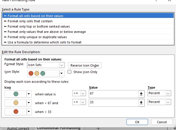
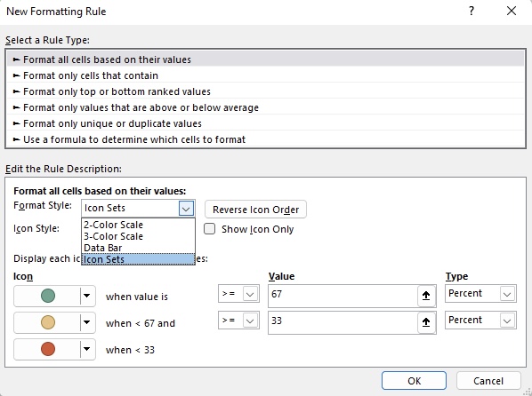
In the Select a Rule Type window, choose Format all cells based on their values.
On the Format Style dropdown arrow, choose Icon Sets.
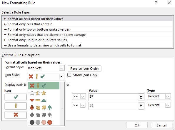
For the Icon Style, choose the check marks and x marks.
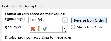
Click on Reverse Icon Order.
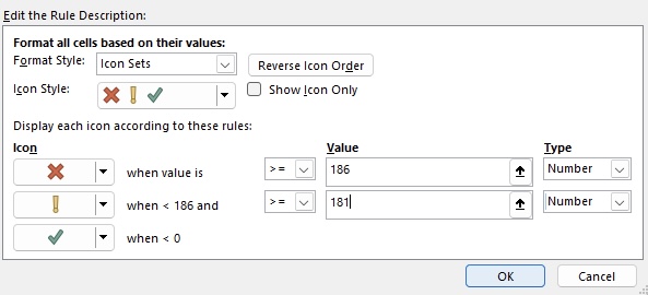
Since we are looking for athletes who have a qualifying time of 180 minutes or less, we will input an X when value is >=181, ! when <186 and >= 181 (meaning it is close but not quite), and ✔ when the value is <=180.
For the Type, choose Number.
Click OK.
Now, the checkmarks will be dynamically inserted in column B. If the value in cell in column B is lesser than or equal to 180, a checkmark will appear.
Inserting Check Mark as an Image
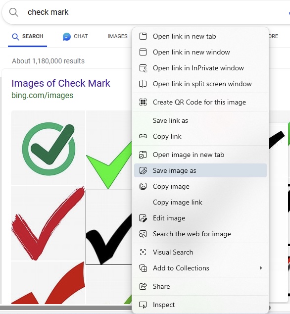
Download a check mark image or create one.
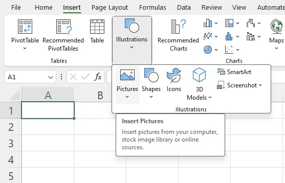
Go to the Insert tab and select Illustrations, then Pictures to insert the image into the desired cell.
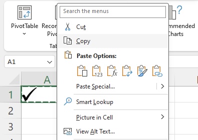
Resize and position the image as needed.
Press CTRL + C to copy, and CTRL + V to paste the image into other cells.
Conclusion:
There you have it! Incorporating check marks into your Excel sheets enhances visual communication and helps in conveying information effectively. Choose the method that best suits your workflow!
John Michaloudis is a former accountant and finance analyst at General Electric, a Microsoft MVP since 2020, an Amazon #1 bestselling author of 4 Microsoft Excel books and teacher of Microsoft Excel & Office over at his flagship MyExcelOnline Academy Online Course.

