Excel Pro Tip: Check Value Exists in Range? Find Out Now!

Check value in Microsoft Excel is essential for data analysis, allowing users to verify data integrity, detect duplicates, and prepare datasets for further examination. Understanding Excel ranges, alongside key functions for identifying values within these ranges, enhances one’s ability to harness Excel’s analytical power efficiently.

Key Takeaways:

• Excel ranges are crucial for various operations, defined by two or more selected cells, enabling users to perform analyses, apply formulas, or execute functions.
• The LOOKUP function offers versatility, allowing for both vertical and horizontal searches within rows and columns to find corresponding values.
• Combining INDEX() and MATCH() functions enhances search accuracy and flexibility, especially beneficial in non-sorted data or complex tables.
• Utilizing COUNTIF for TRUE/FALSE checks provides a straightforward method to verify the existence of specific values within a range, simplifying data validation processes.

 

Getting Started with Excel Range Searches

The Importance of Finding Values in a Range

Finding values within an Excel range is not just about ensuring data integrity; it’s about unlocking the full potential of Excel’s data analytical abilities. Whether you’re reconciling figures, detecting duplicates, or preparing data for further analysis, knowing if certain values exist in a range is a key step in your workflow.

Understanding the Basics of Excel Ranges

Before you dive in, it’s crucial to grasp what an Excel range is. A range in Excel refers to a selection of two or more cells, either adjacent or non-adjacent. These cells can hold values, formulas, or functions that you might need to reference or analyze. Ranges are the building blocks for many operations in Excel and can be defined by their coordinates.

 

Key Functions to Identify Values in Excel Ranges

The Versatility of the LOOKUP Function

The LOOKUP function in Excel is a straightforward tool that lets you search for a value within a row or column and retrieve a corresponding value from another row or column. It’s incredibly versatile because you can use it to look up a value both horizontally and vertically.

Here’s a glimpse of how the function works:

=LOOKUP(Lookup_Value, Lookup_Vector, Result_Vector)

For instance, if you want to find an employee’s age based on their name, you’d set up your lookup and result vectors accordingly:

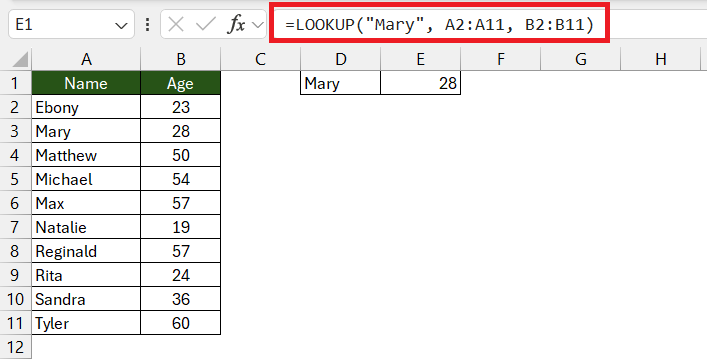
=LOOKUP("Mary", A2:A11, B2:B11)

This formula would scan through column A to find “Mary” and then return the corresponding age from column B.

Remember, LOOKUP assumes that your data is sorted. If it’s not, you might get inaccurate results or an error. So, make sure to sort your data accordingly before you use this function.

 

Harnessing the Power of INDEX() and MATCH()

INDEX() and MATCH() are two of Excel’s most powerful functions and when combined, they can do wonders for range searching. The MATCH function locates the position of a lookup value within a row, column, or table, and the INDEX function then retrieves the value at a given position in a range. This duet offers flexibility and accuracy, especially in non-sorted data or complex tables.

Let’s break it down with syntax and example:

• MATCH: =MATCH(Lookup_Value, Lookup_Array, [Match_Type])
• INDEX: =INDEX(Array, Row_Num, [Column_Num])

To find a specific value using INDEX and MATCH:

=INDEX(Table_Array, MATCH(Lookup_Value, Lookup_Array, 0), Column_Index_Number)

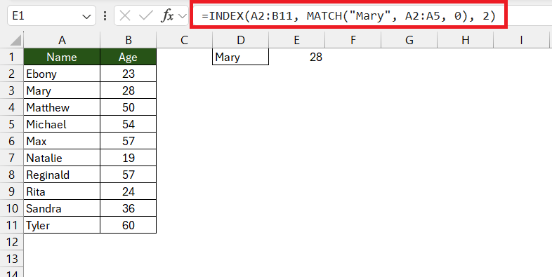
Imagine you need to find the age of “Mary” from our previous example. Here’s how you’d write it:

=INDEX(A2:B11, MATCH("Mary", A2:A5, 0), 2)

The MATCH function searches for “Mary” in column A and returns her position. The INDEX function then grabs the value from the same row in column B, which contains ages.

Understanding these functions can significantly improve your data search capabilities within Excel.

 

Step-by-Step Examples for Common Scenarios

Example 1: Verifying the Presence of a Value with TRUE or FALSE

Let’s tackle a common scenario where you want to check if a specific value exists within a certain range and have Excel confirm it with a simple TRUE or FALSE

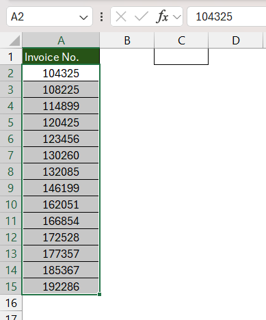
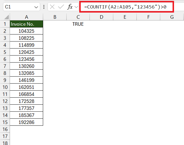
Let’s say you have a list of invoice numbers in cells A1 through A10, and you’re checking for invoice #12345. Here’s an easy step-by-step example using the COUNTIF function:

STEP 1: Identify the range you want to check and the value you’re searching for.

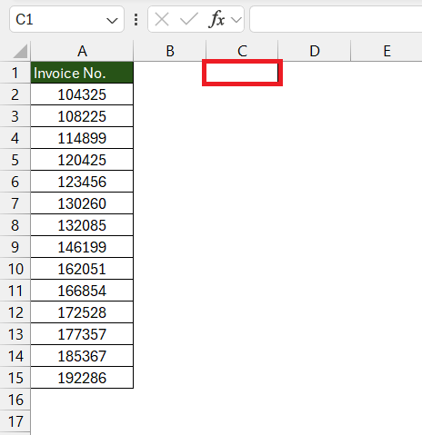
STEP 2: Click the cell where you want the TRUE or FALSE result to appear.

STEP 3: Type in the formula, using the COUNTIF function to determine if the value exists:

=COUNTIF(A2:A15,"123456")>0

• If “123456” is found within the range A2 through A15, the result will return TRUE, indicating presence.
• If not found, it will return FALSE, indicating absence.

This formula provides a quick and efficient way to verify the presence of values without needing to sift through data manually.

 

Example 2: Handling Partial Matches Efficiently

If you’re dealing with a scenario where you only have a fragment of the data you need to match, Excel has got you covered. You can handle partial matches efficiently using the asterisk (*) wildcard in your search criteria. Let’s look at this through a practical example using the COUNTIF function.

For example:

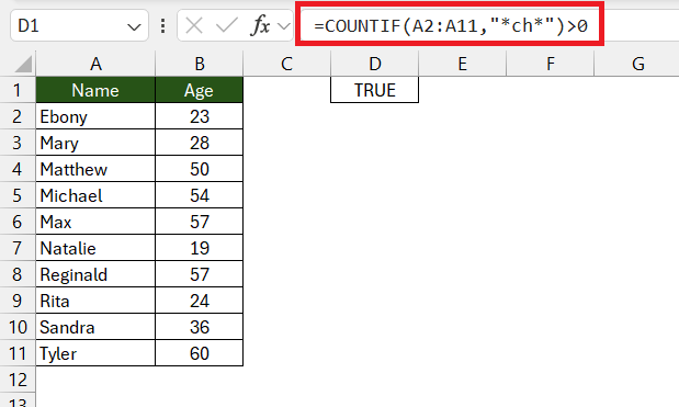
You have a list of team names, and you’re looking for any name that contains the letters “ch”. Here’s the formula you would use:

=COUNTIF(A2:A11,"*ch*")>0

This will return TRUE if any cell within the range A2 through A11 contains the partial match “ch”.

Remember, this is particularly useful when you have data with common prefixes or suffixes, and you need to check for variations of a base term.

 

Advanced Techniques for Range Searching

Combining Functions for Enhanced Searches

Combining Excel functions unlocks potent search capabilities that single functions can’t always offer. By weaving together functions like IF, ISNUMBER, SEARCH, and even logical operators like OR, you can perform intricate searches that answer very specific data questions.

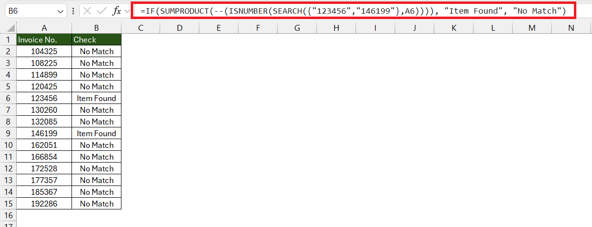
Here’s an example to illustrate combining functions for partial match searches and returning custom results based on findings:

=IF(SUMPRODUCT(--(ISNUMBER(SEARCH({"123456","146199"},A2)))), "Item Found", "No Match")

In this formula:

• SEARCH({"123456","146199"},A2) checks for both “123456” and “146199” within cell A2.
• ISNUMBER(...) evaluates if the SEARCH function returns a numerical position for these strings – indicative of a match.
• SUMPRODUCT(--(...)) adds up the TRUE (converted to 1s) instances to check for any match.
• IF(..., "Item Found", "No Match") is our final evaluator, giving a clear “Item Found” or “No Match” based on the outcome.

Harness the power of combined functions, and you can fine-tune your search to fit very precise requirements, making Excel an even more effective tool for data management and analysis.

 

Tailoring Your Search for Approximate Matches

When exact matches are not required or your data isn’t perfectly uniform, you’ll need to tailor your Excel search to handle approximate matches. This is particularly useful in situations where you’re dealing with ranges or graded data, like tax tables or pricing tiers.

To perform an approximate match, you can use the VLOOKUP or HLOOKUP functions with the range_lookup argument set to TRUE (which is also the default setting).

Here’s a simple syntax for VLOOKUP with an approximate match:

=VLOOKUP(Lookup_Value, Table_Array, Col_Index_Num, TRUE)

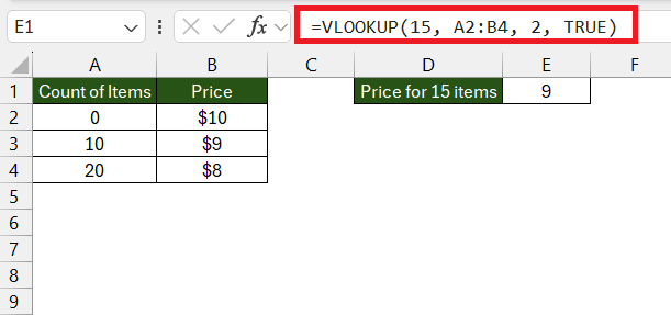
Let’s say you have a pricing tier in which the price reduces as the quantity purchased increases:

• 1-10 items: $10 each
• 11-20 items: $9 each
• 21-50 items: $8 each

If you’re looking to find out how much 15 items cost, you would use:

=VLOOKUP(15, A2:B4, 2, TRUE)

This would return $9 as it finds the closest match without going over the value looked up.

Remember, it’s vital the first column of your table array is sorted in ascending order to make use of approximate matches.

This capability allows for flexibility in your searches and helps cater to datasets that function within defined ranges rather than fixed values.

 

Practical Tips for Error-Free Searches

Debugging Common Errors in Value Searches

When searching for values, running into errors can be a frustrating hurdle. The #VALUE! error in Excel, for example, is a common roadblock that often pops up when something is amiss with your formula or the data it references.

Here’s a breakdown of steps to tackle the #VALUE! issue:

1. Correct Formula Typing: First, ensure your formula is typ`ed correctly and that Excel recognizes the functions and syntax used.
2. Check for Hidden Spaces: Often, #VALUE! errors arise because of hidden spaces. Double-check your cells for any accidental spaces before or after your data.
3. Data Types Matter: Ensure that your formulas aren’t trying to perform operations on data types that aren’t compatible, such as subtracting a number from a text string.

 

Optimizing Performance for Large Data Sets

When working with large data sets, Excel’s performance may slow down, making it necessary to optimize your workbook for efficiency. Here are practical tips for ensuring your value searches run smoothly:

1. Use More Efficient Formulas: Functions like INDEX and MATCH can be better alternatives to VLOOKUP or HLOOKUP because they process only relevant data rather than entire rows or columns.
2. Limit the Use of Volatile Functions: Volatile functions like OFFSET, INDIRECT, TODAY, and RAND are recalculated every time Excel recalculates, which can be resource-intensive. Use them sparingly.
3. Convert Ranges to Excel Tables: This can streamline data management and improve lookup performance. Excel Tables (created using the shortcut CTRL+T) offer structured references and can improve calculation times.
4. Avoid Entire Column References: Instead of using A:A, for instance, restrict the reference to the specific range like A1:A1000.
5. Disable Automatic Calculations: If you’re inputting a lot of data at once, consider setting your workbook to manual calculation mode temporarily (Options > Formulas > Workbook Calculation > Manual).

By applying these optimizations, Excel can process your searches much faster, even when dealing with substantial amounts of information.

Keep in mind that regular maintenance, such as removing unused formulas and compressing the workbook, can further empower your Excel application to handle complex tasks with agility.

 

Frequently Asked Questions (FAQs)

Q1: How do you check if a value is contained in a range in Excel?

You can check if a value is contained in a range in Excel using the COUNTIF function. Enter =COUNTIF(range, "value")>0 in a cell, replacing range with your cell range and value with the value you’re searching for. This will return TRUE if the value is found, FALSE otherwise.

Q2: How do you check if a cell has a value in a spreadsheet?

To check if a cell has a value in a spreadsheet, use the ISBLANK function. Type =ISBLANK(cell) where cell is the cell reference. It returns TRUE if the cell is empty, and FALSE if it contains any data.

Q3: How do I find a specific value in a column in Excel?

To find a specific value in a column in Excel, use the MATCH function. Type =MATCH("value", range, 0) into a cell, where “value” is what you’re looking for and range is the column range. This returns the row position of the value in the column.

Q4: :How do you test for a value in a cell in Excel?

To test for a specific value in a cell in Excel, you can use the IF function in combination with the cell reference. Enter =IF(A1="value", "True", "False") in another cell, replacing A1 with the cell to test and “value” with the actual value you’re looking for. This will return “True” if the cell contains the value or “False” if not.

Q5 :How to use the isnumber excel function?

Use the ISNUMBER function in Excel by typing =ISNUMBER(cell) into a cell, replacing cell with the cell reference you want to check. It will return TRUE if the cell contains a numeric value and FALSE if not. This function is useful for validating data types in your spreadsheet.