How to Use the Excel Match Function

The MATCH function in Microsoft Excel is a powerful tool used to search for a specified item in a range of cells and return the relative position of that item within the range. It is particularly useful for locating the position of an item in a list or array. MATCH can be combined with other functions, such as INDEX, to perform complex lookups and data retrieval tasks. This function enhances efficiency in data analysis and management by streamlining the process of finding and referencing data.

Key Takeaways:

• The MATCH function in Excel searches for a specified item in a range and returns its relative position, aiding in data navigation.
• It is particularly effective for locating items in lists or arrays, enhancing data analysis efficiency.
• MATCH can be combined with functions like INDEX for complex lookups and dynamic data retrieval.
• The function supports different match types (exact, less than, greater than) for versatile searching.
• MATCH is crucial for dynamic, accurate, and time-saving data management in large datasets.

 

Introduction to MATCH Function in Excel

Understanding the Basics of MATCH

The MATCH function in Excel is all about discovery – it’s how you locate the position of a specific item in a list or a range. Think of it as a search tool within your spreadsheet, hunting down the row number where your sought-after data is hunkering down.

The Significance of MATCH in Data Analysis

The importance of the MATCH function in data analysis can’t be overstated. It’s the backbone of searching for crucial data points within massive datasets, enabling you to pinpoint information quickly without slogging through rows and columns.

By using MATCH, you breeze past the manual scrounging and head straight for the insights, enhancing the accuracy of your data analysis and saving precious time. When combined with other functions, MATCH becomes even more potent, allowing for dynamic lookups and versatile data manipulation.

 

The Anatomy of MATCH Function

Syntax Breakdown: How MATCH Works

Understanding the syntax of the MATCH function makes it your trusty companion in navigating Excel’s vast seas of data. Here’s how it works:

=MATCH(lookup_value, lookup_array, [match_type])

• lookup_value: The treasure you’re seeking, be it a number or text; is what you want MATCH to find.
• lookup_array: Consider this the map – the column or row where MATCH begins its quest.
• match_type: This piece of the puzzle determines the nature of the search. It tells MATCH what kind of match to look for – exact or approximate match.

Remember, the MATCH function is like sending out a scout; it reports back with the location, not the value itself. That’s where other functions, like INDEX, join the adventure, turning the location into valuable information.

Match Types Explained: Zero, One, Minus One

Navigating the different match types in Excel’s MATCH function is key to a successful search. Think of the match types as three distinct search modes:

1. When match_type is 1: It’s like using a net to catch the largest fish that isn’t bigger than what you’re looking for. The net – your lookup array – must be arranged from smallest to largest. MATCH will deliver the position of the largest value less than or equal to your needle in the haystack, or in this case, the lookup_value.
2. When match_type is 0: This is the sniper mode for when you need an exact match. No sort order is required; MATCH will scan through the array and lock onto the very first instance that exactly matches the lookup_value.
3. When match_type is -1: If MATCH type 1 is casting a net, this one is for climbing a tree to pluck the smallest piece of fruit that’s still larger than your hand. The caveat? Your list needs to be upside down – sorted in descending order. MATCH finds the smallest value that’s greater than or equal to the lookup_value.

Learning when and how to use these match types can turn you into an Excel search wizard, conjuring the right results with a flick of the MATCH wand.

 

Mastering MATCH with Real-World Examples

Simple MATCH Functions for Everyday Use

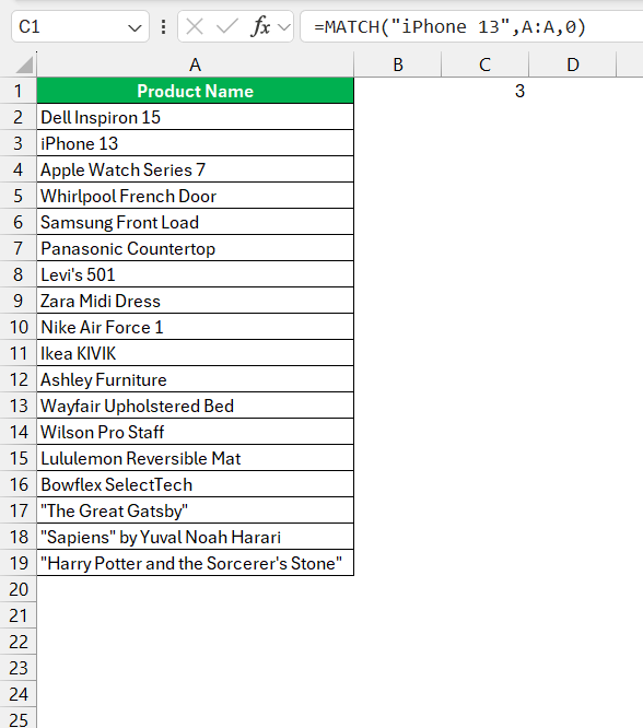
When you roll up your sleeves for the daily data dive, simple MATCH functions are the trusty tools you want in your belt. For the most straightforward tasks, an exact match search (match_type set to 0) is your go-to. This can be incredibly handy for tasks like finding employee IDs in a list or pinpointing a product price in a catalog.

It’s the straightforward, “find-and-report-back” command that turns an overwhelming spreadsheet into a navigable treasure map.

Advanced Scenarios: Using MATCH with Wildcards

For the seasoned Excel explorer, wildcards in MATCH are like a secret weapon. These powerful symbols – the asterisk (*) and the question mark (?) – stand in for unknown characters, unlocking a range of possibilities. The asterisk can replace any sequence of characters, while the question mark steps in for any single one.

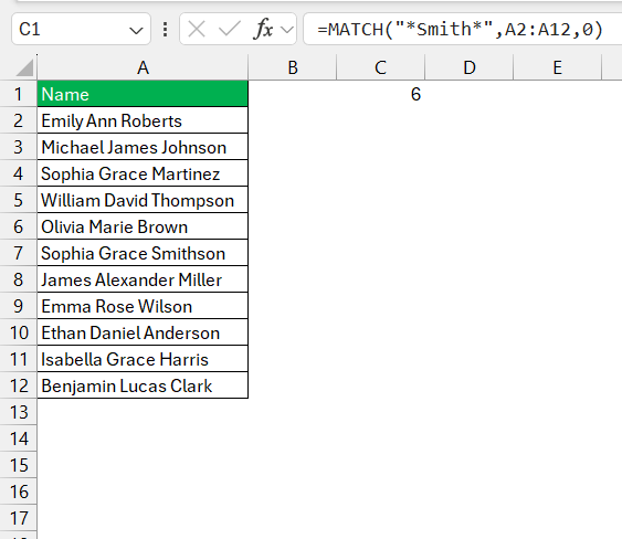
Imagine a situation where you’re sifting through a list of full names to find everyone whose last name starts with “Smith”. A MATCH formula with wildcards makes it a breeze: =MATCH("*Smith*", A2:A12, 0).

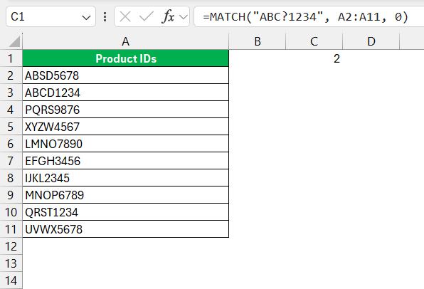
Or, if you have a partial product code and need to discover its full form and position, wildcards come to the rescue again: =MATCH("ABC?1234", A2:A11, 0).

 

Combining Powers: MATCH with Other Functions

Creating Dynamic Lookups with INDEX and MATCH

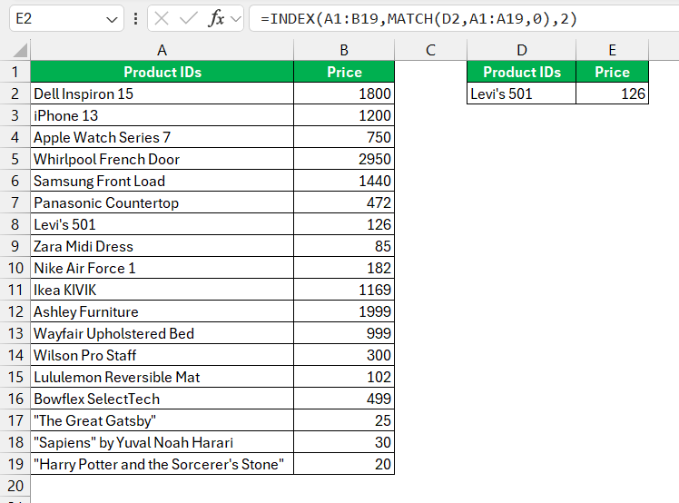
Breaking free from the constraints of single-direction searches, pairing INDEX with MATCH in Excel lets you craft dynamic lookups that would make even the most seasoned data analyst swoon. These dynamic duos dance across rows and columns with grace, fetching values from any cell in a table—regardless of its position.

Imagine you need to pull product prices from a complicated table. With INDEX and MATCH, you can create a formula that adapts to new data like a chameleon, ensuring that your lookups remain accurate and effective no matter how your dataset evolves. This incredible flexibility saves you from the tedious task of updating formulas manually after each data shuffle.

 

Troubleshooting Common MATCH Function Issues

Why Your MATCH Function Might Be Failing

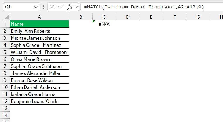
Ever been in that exasperating situation where your MATCH function seems to be on a strike, returning an #N/A error, even though you’re staring right at the value it’s supposed to find? It turns out; that there are a couple of usual suspects behind this mystery.

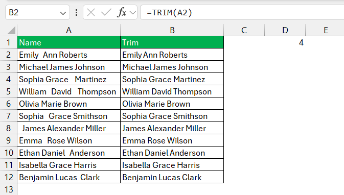
There’s the issue of extra spaces that sneak in, camouflaged either at the beginning, the end, or even doubling up between characters.

Then, those pesky HTML characters — invisible to your eyes but glaring red flags to Excel, throw off the MATCH.

To crack the case, you might play detective with the TRIM and LEN functions or make sure the format of your lookup_value matches that of the lookup_array.

Think of it as getting both parties to speak the same language.

 

FAQ: Mastering the Excel MATCH Function

How do you use match in Excel?

To use MATCH in Excel, you simply write a formula where you specify the value you’re looking for, the range of cells where it might be found, and the type of match you want, exact or approximate. It’ll scout through the cells and report back with the position of the match. It’s a cornerstone for more advanced Excel operations, like dynamic tables and complex data analysis.

What Makes MATCH Different from VLOOKUP?

MATCH offers more flexibility than VLOOKUP by pinpointing the position of a value in any column and not just the first. It’s a tool for position-finding rather than value retrieval, and it excels in accuracy when dataset columns frequently change. VLOOKUP, on the other hand, seeks a value returning the content of a cell, but is more rigid as it requires the value to be in the first column of the table array.

Can MATCH Function Work with Text and Numbers?

Absolutely, MATCH can work its magic with both text and numbers. It’s flexible enough to search for a string of text or numeric values within your data. However, watch out for formatting hiccups—MATCH is keenly aware of the difference between text formatted numbers and actual numeric values, so ensure they’re speaking the same language to avoid errors.

How Do I Update My MATCH Formulas for Entire Column Data?

When your data encompasses an entire column, updating MATCH formulas is a breeze. Simply extend the lookup_array argument to include the whole column. For example, if you’re searching column A, use A:A as your range. Remember, though, for larger datasets, this may slow down your workbook’s performance, so consider limiting the range to the actual data set where possible.

Is There a Way to Perform Approximate Matches with the MATCH Function?

Certainly! To execute approximate matches with the MATCH function, set your match_type argument to 1 or -1. Use 1 when the data is sorted in ascending order, or -1 for descending order. This way, MATCH finds the nearest value less than (with 1) or greater than (with -Ev1) your lookup_value – a useful feature when dealing with ranges or grouped data.