Before I was a Pivot Table guru, I had to get individual rows of daily sales and group them into a report showing the monthly sales during the year.
Group Dates in Pivot Table would take a ton of effort using Formulas: Extracting the month and year from each transactional date; Then manually grouping them together to get the total sales numbers for each month.PAINFUL & SLOW! Thankfully there is the Pivot Table way (I wish I had known this back then), which is quick and reduces the risks of making any errors....ah yeah & I almost forgot, it is also easy to add new data to your sales report with a simple Refresh!
Group Dates in Pivot Table by Month & Year
In the data below, you can see that there are two columns: one that contains the transaction date of the sale, and the second column contains the total sales amount for a particular date.

Want to know How To Group Dates in Pivot Table by Month?
In the example below, I show you how to Pivot Table Group by Month:
STEP 1: Insert a new Pivot table by clicking on your data and going to Insert > Pivot Table > New Worksheet or Existing Worksheet

STEP 2: In the ROWS section put in the Order Date field.
Notice that in Excel 2016 (the version that I am using) it will automatically Group the Order Date into Years & Quarters:

STEP 3: Right-click on any row in your Pivot Table and select Group so we can select our Group order that we want:

STEP 4: We need to deselect Quarters and make sure only Months and Years are selected (which will be highlighted in blue).
This will group our dates by the Months and Years. Click OK.

STEP 5: In the VALUES area put in the Sales field. This will get the total of the Sales for each Month & Year:

This is how you can easily create Pivot Table Group Dates by Month!

Group Dates in Pivot Table by Week
To group the dates by week, follow the steps below:
STEP 1: Right-click on one of the dates and select Group.

STEP 2: Select the day option from the list and deselect other options.

STEP 3: In the Number of days section, type 7.

This is how the group dates in Pivot Table by week will be displayed.

STEP 4: You can even change the starting date to 01-01-2012 in the section below.

Your final grouped data is ready!

Change Formatting
Now we have our sales numbers grouped by Month & Years, notice that we can improve the formatting by following the steps below:
STEP 1:Click the Sum of SALES and select Value Field Settings

STEP 2: Select Number Format

STEP 3: Select Currency. Click OK.

You now have your total sales for each monthly period! Quick & Easy!

Summarize Value by
In the previous examples, you saw how to get total sales by month, year, or week. You can even calculate the total number of sales that occurred in a particular month, year, or week.
Let’s look at an example to know how:
STEP 1: Right-click anywhere on the Pivot Table.

STEP 2: Select Value Field Settings from the list.

STEP 3: In the Value Field Setting dialog box, select Count.

STEP 4: Click OK.

This will summarize the values as a count of sales instead of the sum of sales (like before).

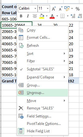
Ungroup Dates
To ungroup dates in a Pivot Table, simply right-click on the dates column and select ungroup.

Or, you can go to the PivotTable Analyze tab and select Ungroup.

Once this is done, the data will be ungrouped again.
Control Automatic Grouping
If you wish to, you can easily turn off this automatic date grouping feature in Excel 2016. To do that, follow the steps below:
STEP 1: Go to File Tab > Options

STEP 2: In the Excel Options dialog box, click Data in the categories on the left.

STEP 3: Check Disable automatic grouping of Date/Time columns in PivotTables checkbox.

STEP 4: Click OK.

This will easily turn off the automatic grouping feature in the Pivot Table! So, the date will be not be grouped automatically now when you drag the date field to an area in the pivot table.
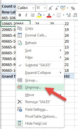
Ungrouping Dates
Automatic grouping can be helpful, but you may need to ungroup dates for detailed analysis. Simply right-click on the dates in the pivot table and choose ‘Ungroup’ from the contextual menu. Alternatively, you could make use of the handy PivotTable Analyze tab and hit ‘Ungroup’.
Frequently Asked Questions
How do I group dates in a pivot table by month and year quickly?
To group dates by month and year in a pivot table swiftly, perform the following steps. First, select any cell containing a date in your pivot table. Next, access Pivot Table Tools, choose ‘Analyze’, followed by ‘Group Field’, and then select ‘Group Selection’. In the dialog box that appears, tick both ‘Months’ and ‘Years’. Once you hit ‘OK’, your dates will be bundled neatly by month and year, revealing an organized overview of your time-based data.
Can you ungroup dates once they have been grouped in a pivot table?
Absolutely! Ungrouping dates in a pivot table is just a few clicks away. Right-click on any date within your grouped data and select ‘Ungroup’. This will restore the dates to their original, ungrouped state, giving you the individual date details you started with. It’s a straightforward process that can be reversed at any time, offering flexibility in your data analysis approach.
How can I practice and become proficient in using pivot tables in excel?
To become proficient in using pivot tables in Excel, practice is key. Start by experimenting with simple datasets, creating pivot tables, and playing with different types of groupings and calculations. Then, watch tutorials, enroll in online courses, or read blogs to learn new tricks and techniques. Gradually move on to more complex datasets. Regularly challenge yourself with new data analysis tasks, and soon, you’ll be navigating pivot tables with ease and confidence.

Bryan
Bryan Hong is an IT Software Developer for more than 10 years and has the following certifications: Microsoft Certified Professional Developer (MCPD): Web Developer, Microsoft Certified Technology Specialist (MCTS): Windows Applications, Microsoft Certified Systems Engineer (MCSE) and Microsoft Certified Systems Administrator (MCSA).
He is also an Amazon #1 bestselling author of 4 Microsoft Excel books and a teacher of Microsoft Excel & Office at the MyExecelOnline Academy Online Course.


