Excel Group by Week Starting on a Monday With Excel Pivot Tables

It is often easier to analyse data when they are grouped by weeks, and creating a Weekly report is super easy in Excel. In this article, we will explore several options to create an Excel group by week table.

Key Takeaways:

• Grouping data by week makes reports easier to read and analyze.
• The WEEKNUM function quickly assigns a week number to each date.
• Pivot Tables can group dates into 7-day periods with just a few clicks.
• You can choose any starting day, such as Monday or Sunday, for weekly reports.
• Data can be ungrouped anytime without affecting the original dataset.

How to Group by Week in Excel

Use WEEKNUM formula

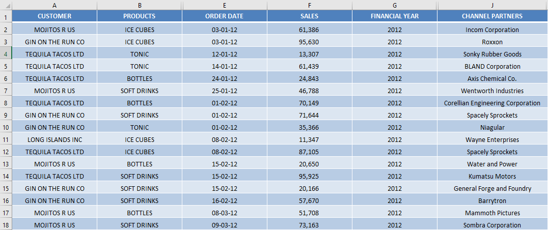
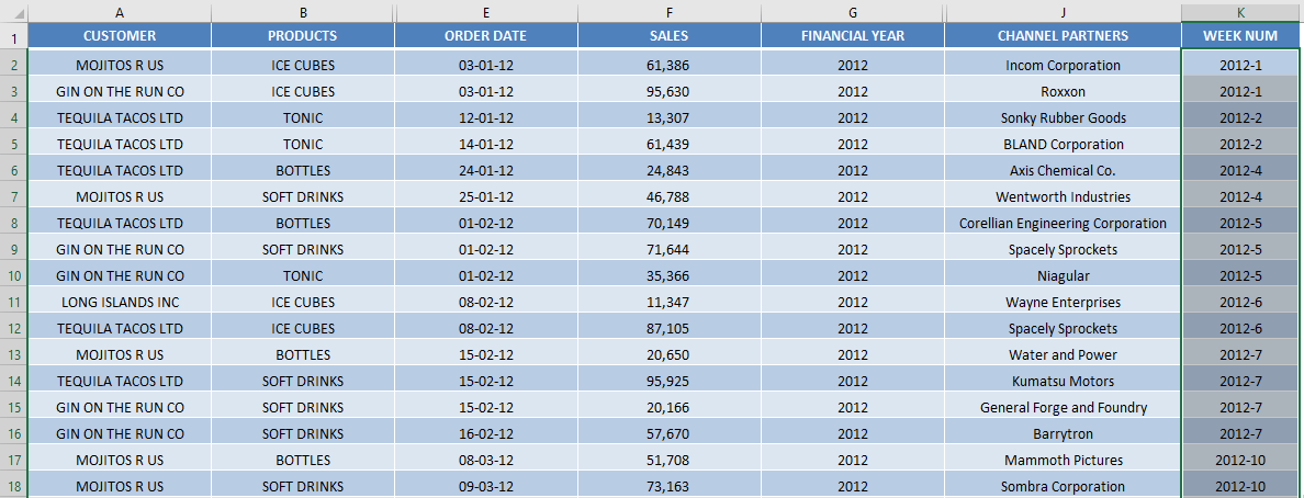
In the screenshot below, you have sales data for a company for which you need to create a weekly report.

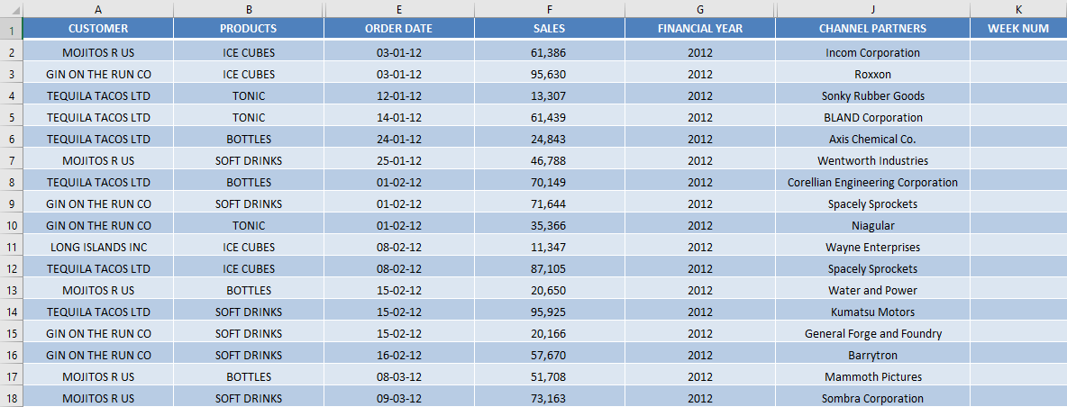
STEP 1: Create a new helper column that will provide the week numbers for the dates.

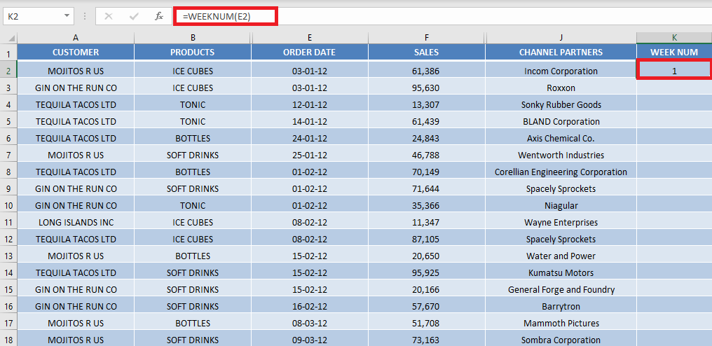
STEP 2: Use the formula – WEEKNUM.  It will simply return the week number of a specified date. By default, Excel will consider that the week begins on Sunday.

STEP 3: This report contains multiple years. Week number should be combined with the year to provide accurate results.

To combine year and week num, use the formula:

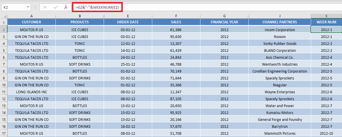
STEP 4: Copy-paste the formula below.

STEP 5: Go to Insert > PivotTable.

STEP 6: In the Create PivotTable dialog box, click OK.

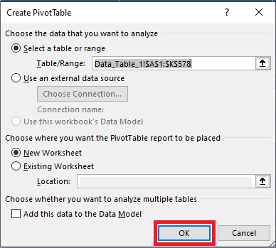
STEP 7: Drag and drop Week Num in the Row field and Sales in the Values field.

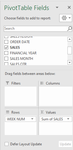
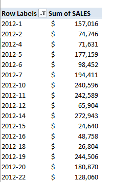
This will provide you with a Weekly Sales Report in Excel using the Weeknum formula.

Using Group Selection

The group selection method will allow you to group by week, starting from any day you choose.

EXAMPLE 1:

STEP 1: Insert a new Pivot table by clicking on your data and going to Insert > Pivot Table > New Worksheet or Existing Worksheet

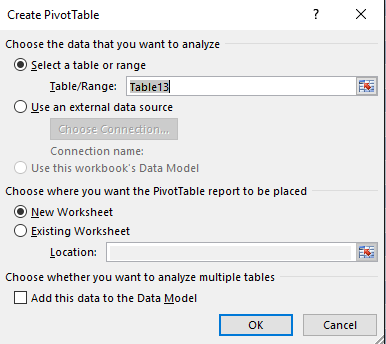
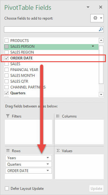
STEP 2: In the ROWS section put in the Order Date field.

Notice that in Excel 2016 it automatically groups dates into Years & Quarters.

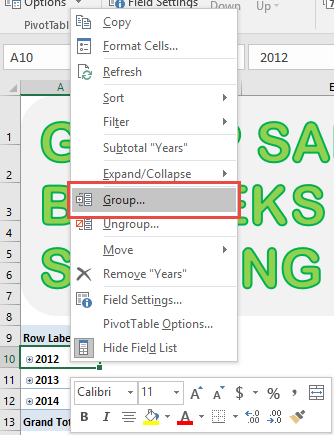
STEP 3: Right-click on any entry in your Pivot Table Row Labels and select Group

STEP 4: Notice that it was able to determine our minimum and maximum dates. However, we need our weeks to start on a Monday.

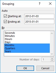
Our starting date is January 3, 2012.  Let us have a quick check-in on our calendar:

We can see that the nearest Monday before that date is January 2, 2012.

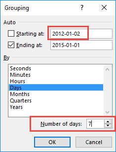
Deselect Months, Quarters, and Years and make sure only Days is selected (depicted by the blue color).

Set the Number of days to 7. 

Set the Start Date as 2012-01-02.

This will Excel group by week (every 7 days starting on a Monday).

Click OK.

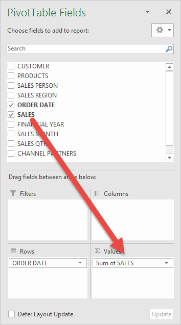
STEP 5: In the VALUES area put in the Sales field.

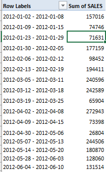
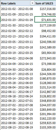
This will get the total of the Sales for each 7-day date range you have defined:

This will create an Excel pivot table group by week!

STEP 6: We can now format our Sales numbers into something more presentable.

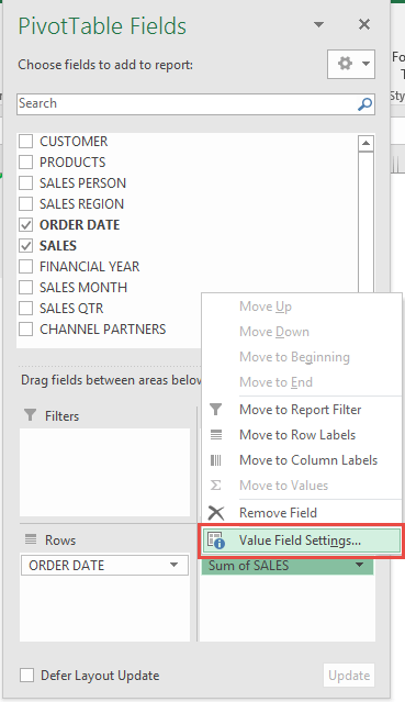
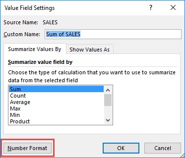
Click the Sum of SALES and select Value Field Settings.

STEP 7: Select Number Format

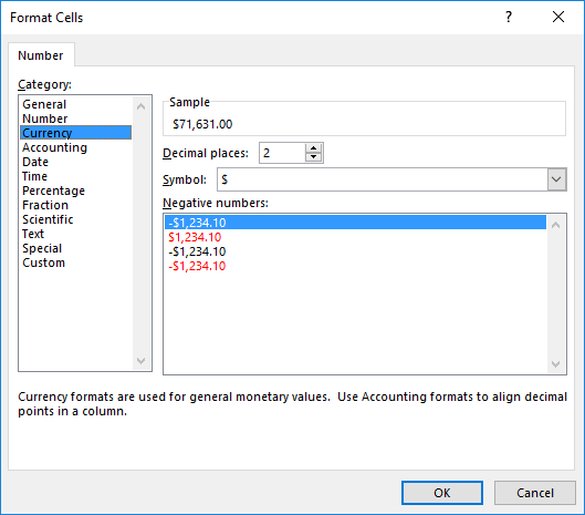
STEP 8: Select Currency. Click OK.

You now have your total sales for each 7-day period starting on Mondays!

EXAMPLE 2:

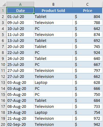
In the example below, there are sales data including sales date, product name, and price sold.

 

STEP 1: Go to Insert > PivotTable.

STEP 2: In the Create PivotTable dialog box, select the table range and new worksheet option, and click OK.

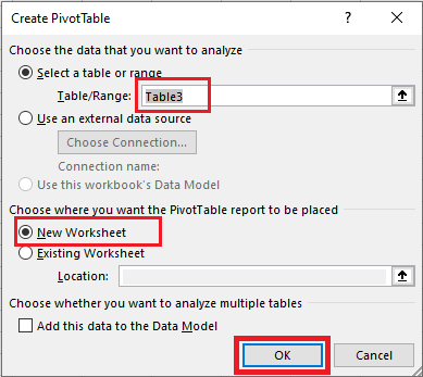
STEP 3: A PivotTable structure will be created in a new worksheet and you can use the PivotTable fields to create a report.

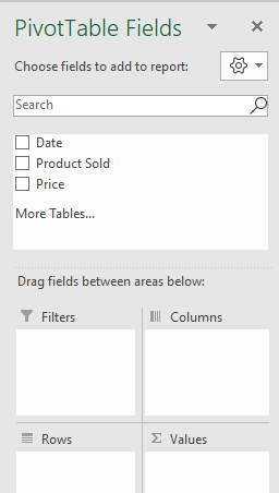
STEP 4: Drag and drop Date in the Row field and Price in the Values field.

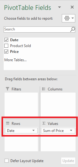
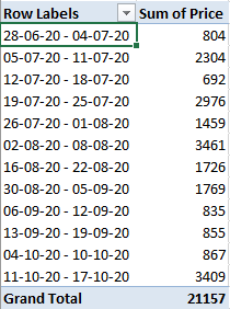
This is how the PivotTable will look like:

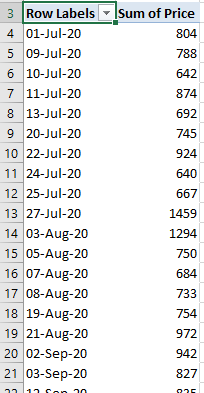
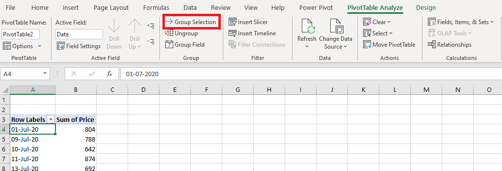
STEP 5: Select any cell in the Date column and then Go to PivotTable Analyze > Group Selection.

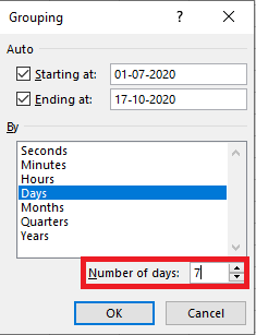
STEP 6: In the Grouping dialog box, select Days (deselect any other option highlighted) and type 7 in the number of days section.

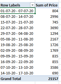
This will group the Pivot Table by a 7-days period.

STEP 7: Type the first Sunday in the given range i.e. 28-06-2020 in this Starting at section.

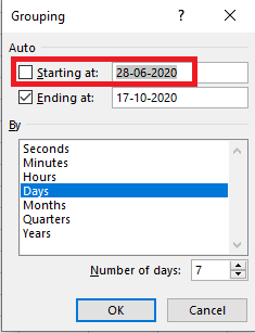
Your weekly sales report starting from a Sunday is now ready!

 

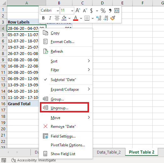
How to Ungroup Data

• Method 1: Right-click on the date column and click Ungroup.

• Method 2: Go to PivotTable Analyze and click on Ungroup.

 

Common Hurdles and How to Overcome Them

Dealing with Irregular Time Spans

When dealing with irregular time spans, your pivot tables might start to look like a patchwork quilt. But fear not, you can smooth out the bumps by ensuring continuous dates are present in your data set. Should you stumble upon a week that defies the norm, consider introducing an artificial data point to maintain consistency. Adjust your grouping to maintain weekly batches, even when there’s a public holiday or a company-specific event that disrupts the regular flow of data. By maintaining a consistent rhythm in your date fields, you’ll ensure your pivot table doesn’t miss a beat.

Navigating Around Blank Cells and Errors

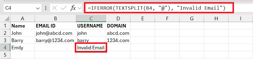
Encountering blank cells and errors can be like hitting roadblocks on your data journey. But with a bit of Excel savvy, you can navigate around them smoothly. Tackle blank cells by locating them with Excel’s Go To Special feature, then decide if you want to plug them with dummy data or simply remove the problematic rows. For errors, IFERROR is your trusty companion, replacing pesky error messages with neutral or zero values, keeping your data looking clean and professional. Remember, a pristine dataset is your ticket to a hassle-free Pivot Table experience.

 

Tips & Tricks

Unlocking Insights with Conditional Formatting

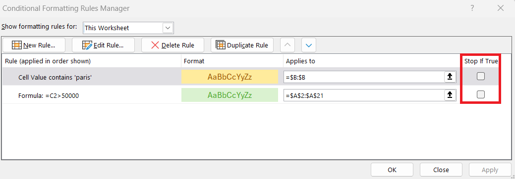
Unlocking insights with conditional formatting is like dabbing color on a monochrome canvas—it brings your data to life. With Pivot Tables, conditional formatting can highlight trends, pinpoint anomalies, and emphasize important figures. Start by applying simple color scales to quickly visualize variations or use data bars for a graphic representation of values. If you’re feeling creative, try applying custom rules to spotlight specific weeks where values exceed targets or dip below benchmarks. Remember, the goal is to make your data not just interpretative but also visually compelling.

Mastering Multiple Date Grouping for Comprehensive Reviews

To become adept at multiple date grouping is to hold the keys to a kingdom of data comprehension. Start off by establishing a solid foundation—group your data by months and years for a sweeping overview. Then, zoom in on the specifics: add layers by grouping by weeks within those months. This technique reveals patterns and trends with a richness and depth that simple date groupings can’t touch. Think of it as viewing your data through a multifaceted lens, where each twist brings a new dimension into focus, offering a comprehensive understanding of fluctuations over time.

 

FAQ

How to group dates by week in Excel?

• Select the data
• Go to the Insert tab and select PivotTable
• Use the Group option with Days set to 7

What does the WEEKNUM function do?

The WEEKNUM formula returns the week number for a given date.

Can I start the week on Monday instead of Sunday?

Yes. Set the desired start date when grouping dates in the Pivot Table.

Why should I combine the year with the week number?

It prevents weeks from different years from being grouped together.

How to remove weekly grouping in a Pivot Table?

• Right-click a grouped date
• Select Ungroup