Match Two Lists With The MATCH Function

You can quickly compare two lists in Excel for matches using the MATCH function, IF function, or highlight the row difference. Manually searching for the difference between two lists can both be time-consuming and prone to errors. You will end up wasting a lot of time! There are various inbuilt functions and features in Excel that can do this task of Excel compare two lists easily.

Key Takeaways

• The MATCH function in Excel can be utilized to determine if a value from one list is present in another, effectively allowing for the comparison of two lists for matching entries.
• If the MATCH function finds a match, it returns the row number of the corresponding item in the second list; when no match is found, it displays #N/A.
• The process can be streamlined by applying the MATCH formula to multiple cells.

Don’t forget to download this Excel Workbook to follow along and compare two lists in Excel for matches:

Highlight Row Difference

You can easily highlight differences in value in each row using the conditional formatting feature in Excel. It will provide you with an idea of how many lines in the columns differ in values.

In the data below, you have two lists in Column A and Column B respectively.

Follow the steps below to highlight row difference:

STEP 1: Select both the columns.

STEP 2: Go to Home > Find & Select > Go To Special or simply press keys Ctrl + G and Select Special to open the Go To Special dialog box.

STEP 3: Select Row Difference and Click OK.

And, Voila!

All the values in Stock List 2 that do not match with the corresponding value in Stock List 1 have been highlighted.

 

STEP 4: You can mark these cells with color as well. Go to Home > Font Color > Select Red.

This will permanently highlight the cells in red font color for future reference.

 

Compare Row using IF function

You can use the IF Function to compare two lists in Excel for matches in the same row. If Function will return the value TRUE if the values match and FALSE if they don’t.

You can even add custom text to display the word “Match” when a criterion is met and “Not a Match” when it’s not met.

Let’s see how we can compare two lists in Excel for matches using IF Function:

STEP 1: We need to enter the IF function in a blank cell.
=IF(

STEP 2: Enter the first argument for the IF function – Logical_Test

What is your condition?

The value in cell D12 is equal to the value in cell C12.
=IF(D12=C12,

 

STEP 3: Enter the second argument for the IF function – Value_if_true

What value should be displayed if the condition is true?

The text displayed should be Match if D12 is equal to C12.
=IF(D12=C12,"Match",

 

STEP 4: Enter the third argument for the IF function – Value_if_false

What value should be displayed if the condition is false?

The text displayed should be Not a Match if D12 is not equal to C12.
=IF(D12=C12,"Match","Not a Match'')

 

STEP 5: Apply the same formula to the rest of the cells by dragging the lower right corner downwards.

 

Compare List using Match Function

Before we understand how to compare two lists in Excel for matches, let’s first go through the basics of what the MATCH function Excel does.

 

What does it do?

It returns the position of an item in a range.

Formula breakdown:

=MATCH(lookup_value, lookup_array, [match_type])

What it means:

=MATCH(lookup this value, from this list or range of cells, return me the Exact Match).

---

I am sure that you have come across many occasions where you have two lists of data and want to know if a specific item in List1 exists in List2.

Well, I have!

With the MATCH function, you can verify if a cell´s item in List1 exists in List2.

The function will return the row position of that item in List2 hence confirming that it exists.  If you get a #N/A it means that the cell´s item does not exist in List2.

You can then go ahead and filter your List1 with either the values returned or the #N/As.

Here are our 2 Lists:

STEP 1: We need to enter the MATCH function in a blank cell:
=MATCH(

 

STEP 2: Enter the first argument for the MATCH function – Lookup_value

What is the value you want to check?

Select the cell containing the List1 value, as this is what we want to check against List2.
=MATCH(C12,

 

STEP 3: Enter the second argument for the MATCH function – Lookup_array

What is the list you want to check against?

Select the entire List2.

And ensure to press F4 to make it an absolute reference.
=MATCH(C12, list2!$C$12:$C:21,

 

STEP 4: Enter the third argument for the MATCH function – Match_type

How specific is your matching? We want an exact match so place in 0.
=MATCH(C12, list2!$C$12:$C:21, 0)

 

STEP 5: Apply the same formula to the rest of the cells by dragging the lower right corner downwards.

 

You now have all of the results!

You can see which row numbers the items exist in List2. For example, Mon45657 in List1 exists in List2 Row 9! If it does not exist in List2, then #N/A is displayed.

 

Using either of the three ways mentioned in this article, you can easily compare two lists in Excel for matches!

 

FAQ: Frequently Asked Questions

Can I Find Partial Matches with the MATCH Function in Excel?

Yes, even though the MATCH function itself looks for exact matches by default, you can gear up Excel to seek out partial matches. This can be a game-changer when working with data that contains similar but not identical entries. You can use the wildcard characters, the asterisk (*) and the question mark (?), for partial matches.

For instance, if you’re comparing company names, and you want to find “JPMorgan” even when it’s listed as “JPMorgan Chase,” an asterisk can help: =MATCH("*"&"JPMorgan"&"*", Range, 0)

The asterisks tell Excel to find any cell where “JPMorgan” appears, surrounded by any number of characters. Just remember, MATCH and wildcards can be a slightly more complex combination, so be extra mindful of what you’re looking for to prevent inaccurate matches.

What Are Some Alternatives to the MATCH Function for Comparing Lists?

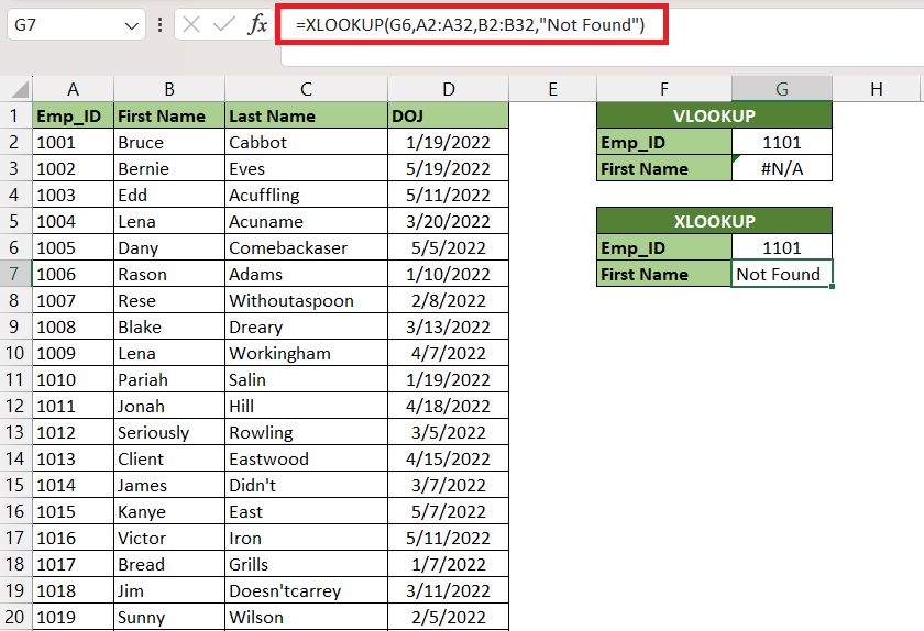
While the MATCH function is quite the tool for comparing lists in Excel, one size doesn’t fit all in the data analysis wardrobe. Depending on the task at hand, VLOOKUP, INDEX, and the newer XLOOKUP might better suit your needs.

VLOOKUP takes a lookup value and scans down the first column of a specified range to return a value from the same row. It’s great when you need more than just the position and want the actual data. However, it’s limited to searching only to the right.

INDEX and MATCH can be paired for more flexibility, with INDEX returning the value at a specific location in a range, and MATCH providing the row or column number.

And XLOOKUP can look in any direction—up, down, left, or right—and it handles missing values more gracefully.