Learning to find multiples of 16 in Microsoft Excel is useful for various tasks in finance, education, and data analysis. Recognizing these patterns can boost your efficiency and accuracy. Excel’s powerful functions simplify complex calculations, especially with large datasets. This guide will cover essential techniques for mastering multiples of 16 in Excel.
Key Takeaways:
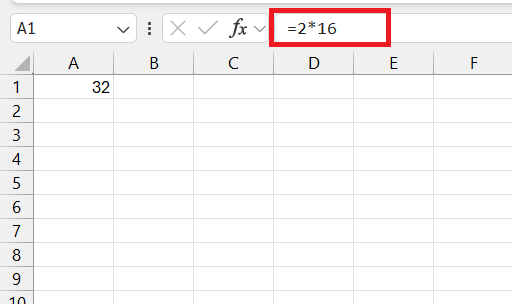
- Use the multiply symbol (*) for basic multiplication. Typing =2*16 in a cell calculates the second multiple of 16, giving you 32.
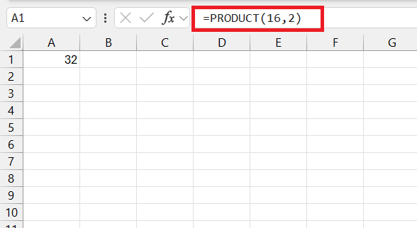
- The PRODUCT function multiplies multiple numbers or cell references. For example, =PRODUCT(16, your_other_number) multiplies 16 by the specified number or cell reference.
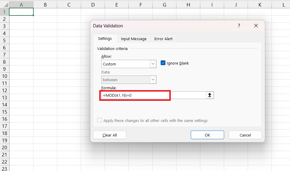
- The MOD function ensures only multiples of a specific number are entered. Using =MOD(A1,16)=0 in data validation restricts entries to multiples of 16.
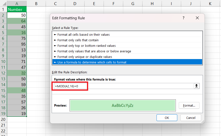
- Apply conditional formatting with the MOD function to highlight multiples of 16 in a dataset. Use =MOD(A1,16)=0 to format cells containing multiples of 16.
Table of Contents
Introduction to Multiples of 16 in Excel
The Importance of Finding Multiples
Understanding the concept of multiples, especially multiples of 16, can be essential for various computational tasks. Whether you’re in finance, education, or simply dabbling in data analysis, recognizing patterns and sequences like these can streamline processes, provide insights, and even help with forecasting and budgeting.
Excel as a Tool for Multiplication Mastery
Excel is not just a spreadsheet tool; it’s a powerhouse for calculations, allowing you to become a master of multiplication with ease. With its versatile formulae and functions, Excel can quickly find the multiples of any number, including 16. This can be particularly beneficial when dealing with large datasets where manual calculation is not feasible.
Setting the Stage for Multiplication
Basic Multiplication in Excel
To get started with basic multiplication in Excel, all you need is the multiply symbol (*). Imagine you want to quickly calculate a series of multiples of 16. You can start by typing ‘=’ in a cell, followed by your starting number and an asterisk, then 16. Press Enter, and Excel will display the result. For instance, typing =2*16 would give you the second multiple of 16 i.e. 32.
Understanding Cell References in Formulas
Cell references in Excel are crucial as they dictate how your formulas will react when copied or moved across your worksheet. Cell references in spreadsheets can be categorized into three types: relative, absolute, and mixed.
A relative reference, like A1, adjusts when the formula is copied to another cell, changing according to its relative position. An absolute reference, such as $A$1, remains constant regardless of where it is copied, locking both the column and row. Mixed references, like A$1 or $A1, lock either the column or the row, allowing for partial adjustment when the formula is copied.
By understanding these references, you can control the behavior of your formulas and ensure they’re referencing the correct cells. Taking the time to grasp how these work will save you a lot of headaches down the line!
Finding Multiples of 16 with Formulas
Using the PRODUCT Function
When your heart is set on calculating products in Excel, the PRODUCT function is your go-to tool. It’s a straightforward method that lets you multiply a series of numbers or cell references effortlessly. Want to find multiples of 16? Just type =PRODUCT(16, your_other_number) in the function, replace “your_other_number” with the cell reference or actual number you want to multiply by 16.
Remember, you can include up to 255 numbers or cell references within the PRODUCT function, making it highly versatile for complex calculations.
Incorporating the MOD Function for Validation
Now, here’s a neat trick when you’re eyeing to ensure that only multiples of a specific number are entered in your Excel sheet: the MOD function. This function returns the remainder after a number is divided by a divisor. To limit entries to multiples of 16, you can use data validation with a custom formula: =MOD(A1,16)=0.
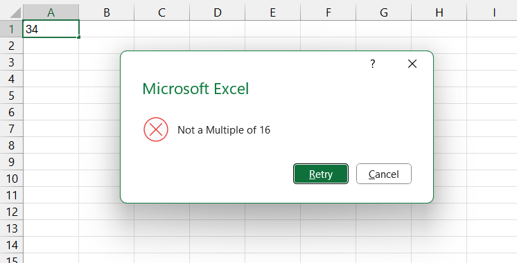
This would allow only values that, when divided by 16, leave no remainder, guaranteeing they’re multiples. If users try to enter anything else, they’ll get a prompt letting them know about the error.
Crafting More Complex Calculations
Conditional Formatting for Identifying Multiples
If you’re looking to quickly identify multiples of 16 in a dataset, conditional formatting is your best friend. By applying a rule that highlights cells using the MOD function—MOD(A1,16)=0—any cell containing a multiple of 16 can be made to stand out with your chosen formatting style.
Just like that, your data becomes much easier to navigate and analyze.
Practical Scenarios for Using Multiples
Real-World Examples in Business and Finance
In the realm of business and finance, competitors who leverage multiples of 16 might have an edge. This could be as straightforward as computing discounts on bulk orders—where pricing might be set at multiples of 16—or complex amortization schedules where payments align with specific intervals. With Excel, these calculations become seamless and instantaneous, providing a solid platform for financial analysis and budgetary planning.
Educational and Training Applications
Educators and trainers find Excel a worthwhile ally, especially when illustrating concepts of multiplication and number sequences. By using Excel to find and visualize multiples of 16, they can offer hands-on experience in mathematical principles and computer literacy. In settings where learning Excel itself is the goal, exercises centered on multiples can provide practical examples for students to hone their spreadsheet skills.
FAQs
How to do multiples in Excel?
To find multiples of a number in Excel, enter =ROW() * your_number in a cell and drag the fill handle down. Replace “your_number” with the desired multiple, such as 16 for multiples of 16.
How to get multiples of 5 in Excel?
To get multiples of 5 in Excel, you can use a simple formula: =(ROW()-1)*5. Start this in the first cell of your column and drag down to fill the series. This will create a sequence of multiples of 5.
How do you round to a multiple of 3 in Excel?
To round to the nearest multiple of 3, use the MROUND function by typing =MROUND(your_number, 3). Replace “your_number” with the cell reference or actual value you want to round.
How do I multiply an entire column by 16?
To multiply an entire column by 16, enter =C2*16 in the first cell beside your column and fill down. Remember to replace C2 with the cell that contains your first number. Use the fill handle to apply it to the rest of the cells quickly.
Can I automatically highlight all multiples of 16 in a range?
Yes, you can automatically highlight all multiples of 16 in a range using conditional formatting. Select your range and go to ‘Conditional Formatting‘ > ‘New Rule. Choose ‘Use a formula to determine which cells to format’ and input =MOD(your_cell, 16) = 0, then set your desired format.
John Michaloudis is a former accountant and finance analyst at General Electric, a Microsoft MVP since 2020, an Amazon #1 bestselling author of 4 Microsoft Excel books and teacher of Microsoft Excel & Office over at his flagship MyExcelOnline Academy Online Course.

