Group By Quarters and Years With Excel Pivot Tables

In the example below I show you how to add quarters to pivot table in Excel:

STEP 1:Insert a new Pivot table by clicking on your data and going to Insert > Pivot Table > New Worksheet or Existing Worksheet

STEP 2: In the ROWS section put in the Order Date field.

Notice that in Excel 2016 (the version that I am using) it will automatically Group the Order Date into Years & Quarters:

STEP 3:If you do not have Excel 2016, right-click on any Row value in your Pivot Table and select Group 

STEP 4:In the Grouping dialogue box, Excel was able to determine our date range (minimum date and maximum date).

Make sure only Quarters and Years are selected (which will be highlighted in blue).

This will group Excel pivot table quarters. Click OK. 

Notice that a Years field has been automatically added to our PivotTable Fields List.  This is cool, as we can use this field for further Pivot Table analysis:

STEP 5: In the VALUES area put in the Sales field. This will get the total of the Sales for each Quarter-Year date range:

Now we have our sales numbers grouped by Years & Quarters!

Notice that we can improve the formatting:

STEP 6: Click the Sum of SALES and select Value Field Settings

STEP 7: Select Number Format

STEP 8: Select Currency. Click OK.

This is how to add years and quarters to Pivot Table. You now have your total sales for each quarterly period!

Common Pitfalls and How to Avoid Them

Dealing with Blank Cells and Text Issues

It’s a common issue that can prevent you from grouping your data effectively. If a date or number field contains blanks, simply fill in those cells with a date or number—feel free to use a placeholder if necessary. For text stumbling in where numbers should be, whisk them away or convert them to actual numbers using Excel’s built-in functions.

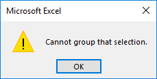
Handling ‘Cannot Group That Selection’ Errors

If you get this error, the cause might be that your pivot table was added to the Data Model, which requires a uniform data type for grouping. Try creating a new pivot table without adding it to the Data Model. If previous groupings linger in your field list, clear them out to start again.

Frequently Asked Questions

How do I group dates by month and year in a pivot table?

To group dates by month and year in a pivot table, first ensure that all cells in your date column are correctly formatted as dates. Select any date in the pivot table, go to ‘PivotTable Analyze’ tab, click ‘Group Field’, select ‘Months’ and ‘Years’, and click OK.

Why am I unable to group selected data in my pivot table?

If you’re unable to group selected data in your pivot table, the problem might be due to non-date values or blanks in your date column, or perhaps your pivot table is part of the Data Model which doesn’t permit grouping. Another way is to recreate the pivot table without adding it to the Data Model to enable grouping.