How to Add 36 Months from Today in Excel – Date Calculations Guide

Adding 36 months from today in Microsoft Excel is a straightforward process that involves the use of the EDATE function, a powerful tool for date arithmetic in financial models and time-sensitive calculations. This task can be accomplished by simply inputting the current date and utilizing a formula to project the date three years into the future. The steps are designed to be user-friendly and efficient, making date extensions in your Excel spreadsheet a hassle-free experience.

Key Takeaways

• Use the =EDATE function with today’s date by inputting =EDATE(TODAY(), 36) to add 36 months from today.
• Ensure the starting cell is formatted as a Date by pressing Ctrl + 1 and selecting the Date category.
• Input the number 36 in a separate cell to indicate the number of months to add if you prefer to reference cells in the formula.
• Confirm the output cell where the future date is displayed is also formatted as a Date to avoid seeing a serial number.

 

Download Excel Workbook and follow along with the tutorial on how to Add 36 months from Today in Excel – Download excel workbook36-months-from-now.xlsx

 

The Power of Date Calculations in Excel

Microsoft Excel is not just a tool for crunching numbers and storing data; it provides a robust platform for managing and analyzing time-based information. Effective date calculations enable businesses, researchers, and individuals to track progress, forecast trends, and manage schedules. Whether you’re calculating loan payment due dates, projecting future sales, or simply planning an event, date functions in Excel give you the power to navigate time with precision.

Why Adding Months Matters in Your Data Analysis

Adding months to date fields in Excel can significantly enhance your data analysis by allowing for thoughtful planning, forecasting, and trend recognition. For businesses, this might involve doing financial modeling to project future revenues or expenses and adjusting to different time periods. For example, being able to quickly forecast monthly financial models requires the ability to add one month incrementally to a start date. If the analysis calls for a quarterly review, being able to add three months at a time can be invaluable for efficiency and accuracy.

Education professionals might use this function for setting up academic calendars, while project managers may rely on it for milestone tracking in their project timelines. In personal use cases, adding months is instrumental when calculating the expected date for significant life events, like maternity leave, loan payoffs, or investment maturities. In each scenario, being able to manipulate and predict dates accurately can be the key to making informed decisions and maintaining control over future events and obligations.

 

Navigate the Time Tunnel in Excel

Excel’s Date Function: A Primer

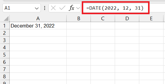
Excel’s DATE function is fundamental for anyone looking to perform date calculations. This function lets you craft a date by defining three separate components: the year, the month, and the day. Each of these is inputted as an argument in the function. For instance, the formula =DATE(2022, 12, 31) will return the date of December 31st, 2022. Here’s what you need to know about the DATE function’s structure:

• YEAR: A four-digit number representing the year.
• MONTH: A numeric value between 1 (January) and 12 (December) symbolizing the month.
• DAY: A numeric value, contingent on the month’s number of days, representing the day of the month.

The beauty of the DATE function lies in its flexibility to operate with both static dates and cell references containing date components. This dynamic function becomes indispensable when creating timelines, expiration dates, or schedules in Excel. Its mechanism minimizes errors, as Excel will automatically rectify any ‘rollovers’ (for example, if you add 13 months, Excel will increment the year).

Understanding and utilizing the DATE function correctly serves as a stepping stone to more advanced date manipulation in Excel.

 

Meet EDATE: Your Shortcut to Future Dates

Excel’s EDATE function is a sleek and purposeful tool designed to streamline your time-traveling tasks in spreadsheets. It has a straightforward objective—add or subtract a specific number of months to or from a given date—and execute this with minimal user input.

The syntax of the EDATE function is concise:

Where start_date refers to the baseline date from which you wish to travel in time, and months represents the number of months you plan to navigate into the future or the past. Interestingly, these values can be provided directly, like =EDATE("2023-01-01", 36), or with cell references that contain the date and the number of months.

An important thing to note is that months can be a positive value to move into the future, or a negative one to step back into the past. And when Excel does its magic, you will see your newly calculated date, landing on the corresponding day of the intended month. So, if you add one month to January 15, 2023, you’ll arrive at February 15, 2023—unless, of course, you’re dealing with the anomalies of leap years or months with fewer days, in which case Excel smartly adjusts the date to the last valid day of the month.

EDATE shines when applied to tasks like projecting deadlines, setting schedules, and ensuring compliance with time-bound scenarios, such as warranty periods or subscription durations. It’s a simple yet mighty function that augments your temporal arsenal in Excel.

 

Putting Excel to the Test: Adding 36 Months

Automated Time Travel: Using EDATE for Quick Results

Using EDATE for quick date calculations is like having a time machine at your fingertips that harnesses the precision of automation. This level of automation not only saves you time but also reduces potential errors that could occur when manually calculating future or past dates.

Imagine you’re tasked with adding exactly 36 months from today’s date for a long-term planning strategy. The EDATE function delivers immediate results without having you count each month on your calendar. Here’s how you can achieve automated time travel in Excel with EDATE:

For directly using today’s date in the formula:

Or, if you have a specific start date in a cell (A2, for instance), you can reference it like this:

Upon entering either formula, Excel returns the date that falls 36 months after the start date specified, positioning you exactly three years into the future with zero hassle.

For those occasions where you require a date in the past, you just need to include a negative number as the month argument:

This would take you 36 months back from the start date in cell A2.

 

Crafting Custom Formulas: Combining Functions for Precision

When standard functions like EDATE don’t fully satisfy complex or unique date calculation needs, crafting custom formulas by combining multiple Excel functions becomes a powerful excel strategy.

Suppose you need a more intricate date calculation, such as adding 36 months, 15 days, and excluding weekends. This would require a concoction of Excel functions:

1. EDATE to add months,
2. DAYS to add specific days, and
3. WORKDAY to exclude weekends or holidays.

Here’s how a sophisticated formula might come together:

In this example, B2 contains the start date, 36 is the number of months to add, and 15 is the number of days to add. The $A$2:$A$4 would be a range of cells that include dates of holidays, which you’d also like to exclude from your calculation.

By understanding the purpose and power of each function, you can tailor a solution that closely aligns with your specific temporal needs. This type of precision ensures that you’re not merely approximating dates, but accurately modeling and forecasting based on exact criteria.

Combining these functions not only enhances the accuracy but also amplifies the overall utility of your Excel toolkit. With a little experience and experimentation, you can navigate even the most complex time-based scenarios with confidence.

 

Streamline Your Workflow: Tips and Tricks

Keyboard Shortcuts: Speed Up Your Date Calculations

Maximizing efficiency in Excel often comes down to the swift use of keyboard shortcuts. They can save you from the tedium of repeated mouse clicks and significantly speed up your work with date calculations. A handful of shortcuts can make dealing with dates in Excel substantially quicker:

1. Ctrl + ; (Semicolon): This shortcut instantly inserts today’s date into the selected cell. It’s particularly handy when you’re logging current dates without the hassle of manual entry.
2. Ctrl + Shift + #: Applying this shortcut after selecting a cell will format the cell to display the default date format. If you’ve just performed a calculation that returns a date serial number, this shortcut will quickly render it in a legible date format.
3. Ctrl + Shift + Arrow keys: If you need to select a range of cells with date values for formatting or applying functions, this shortcut will extend the selection from the current cell to the last nonblank cell in the specified direction.
4. Ctrl + Shift + ~: This reverts the formatting of a cell back to the general number format. It’s useful when you need to see the underlying date serial number or if you’re troubleshooting unusual date behaviors.

Each of these shortcuts serves as a cog in the well-oiled machine that is your workflow, reducing steps and enabling smooth date and time manipulations. As you become more familiar with them, you’ll notice a substantial increase in your work efficiency, freeing you up to focus on the analysis and interpretation of your date and time data rather than the input and formatting processes.

 

Conditional Formatting: Visual Cues for Time-Based Data

Conditional Formatting in Excel is akin to an artist adding color to a canvas—it brings attention to critical elements, communicates status, and makes patterns immediately visible. When it comes to time-based data, conditional formatting enriches your spreadsheets by providing visual cues that can help you quickly assess temporal information.

For example, let’s say you want to track project deadlines. By using conditional formatting, you can set rules to color-code dates that are approaching, past due, or completed within certain time frames. Adding these visual markers improves readability and allows you to prioritize tasks or identify issues at a glance.

Here’s how you can apply conditional formatting to your date calculations:

• Highlight Cells Rules: By going to Home > Conditional Formatting > Highlight Cells Rules > A Date Occurring, you can select various periods relative to the current date, like “Next Month”, “Last Week”, etc., to add automatic coloring to cells based on these criteria.

• Using Formulas: For more control, use formulas in conditional formatting. For instance, to highlight dates 3 months from now, select your range of dates, go to Conditional Formatting > New Rule > Use a formula to determine which cells to format, and input a rule such as:

By combining the DATE and EDATE functions with conditional formatting, you turn your spreadsheet into an intuitive, visually-guided dashboard that aids in the effective management of your schedules, deadlines, and any time-sensitive data.

 

FAQ: Time-Related Queries Clarified

How do I calculate 36 months from a date in Excel?

To calculate 36 months from a specific date in Excel, you can effectively use the EDATE function. This function takes a start date and the number of months you want to add as arguments, giving you the date that is 36 months later.

How do I calculate months from today in Excel?

To calculate a certain number of months from today’s date in Excel, you would once again call upon the EDATE function, but this time in combination with the TODAY function, which fetches the current date.

How Do I Ensure Accurate Date Calculation Across Different Years?

Stick to using Excel’s built-in date functions like DATE, EDATE, DATEADD, DATEDIF, and TODAY, which are designed to handle date calculations accurately, taking into account leap years and differing numbers of days in each month.

How to update the years as months are added?

To update the years as months are added in Excel, you can use the EDATE function with a formula that multiplies the number of years by 12 to convert them into months. For example, to add years to a date in cell A2, use the formula `=EDATE(A2, B2*12)` where B2 contains the number of years you want to add, which the formula will multiply by 12 to convert to months, thus updating the years accordingly. Ensure the resulting cell is formatted as a Date to display the updated year.