50 Things You Can Do With Excel Pivot Table

Want to know how to use Excel Pivot Tables, Slicers, Charts and Dashboards?

1. Tables

Excel Tables are very powerful and have many advantages when using them. You should start using them asap regardless of the size of your data set, as their benefits are HUUUGE:

1. Structured referencing;
2. Many different built-in Table Styles with color formatting;
3. Use of a Total Row which uses built-in functions to calculate the contents of a particular column;
4. Dropdown lists that allow you to Sort & Filter;
5. When you scroll down from the Table, its Headers replace the Column Letters in the worksheet;
6. Remove Duplicate Rows automatically;
7. Summarize the Table with a Pivot Table;
8. Supports calculated Columns so you can create dynamic formulas outside the Table;

STEP 1: Select a cell in your table

STEP 2: Let us insert our table! To do that press Ctrl + T or go to Insert > Table:

STEP 3: Click OK.

Your cool table is now ready!

2. Inserting a Pivot Table

Pivot Tables in Excel allow you to analyze thousands of rows of data with just a few mouse clicks. It is the most powerful tool within Excel due to its speed and output and I will show you just how easy it is to create one.

If you are using a table or data set to analyze your information, then you should always use a Pivot Table which will enhance your analytical capabilities as well as save you heaps of time off your daily routine.

They are used by Project Managers, Finance Analysts, Auditors, Cost Controllers, Sales Analysts, Financial Controllers, Human Resources, Doctors, and Statisticians just to name a few. Heck, I even created an in-depth online course on Pivot Tables, that’s how in demand this Excel tool is in right at this moment!

STEP 1: Click in your dataset.

STEP 2: Go to Insert > Pivot Table

STEP 3: Place the Pivot Table in a New or Existing Worksheet

STEP 4: Drag and Drop the fields

You now have your Table ready!

3. Drill down to audit

When you are using a Pivot Table in Excel and want to know what data makes up a certain value, all you have to do is double click on that cell.

This will open up a brand new Sheet with all the rows of data that make up that value.

NB. This is an extraction of your data source, so if you edit the information and Refresh your Pivot Table then nothing will happen. Any changes need to be made in your main data source.

If you want to get rid of this sample data, all you have to do is press CTRL+Z and press DELETE in the popup box.

So go ahead and double click on any values (including SubTotals and GrandTotals) within your Table to view the data that makes up your selected value.

STEP 1: Double click on any value cell within the Pivot Table

This opens up a new sheet with the data that makes up the selected cell.

Note: You can change the data that is in this new sheet but that will not affect the Table or your original data source.

4. Refresh

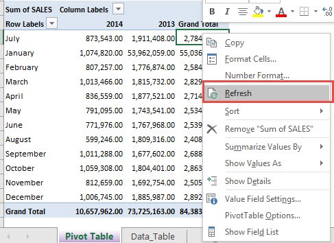
When the information in your data set gets updated you need to Refresh your Pivot Table in Excel to see those changes in your Pivot Table. There are three ways to do this. First click on your Table and:

1. From the Ribbon choose: PivotTable Tools > Options > Refresh

2. Press ALT+F5

3. Right-click in your Table and choose Refresh (see this option below)

STEP 1: Change the information in your data set.

STEP 2: Click on the Pivot table.

STEP 3: Right-click and select Refresh.

Your values in the table are now updated!

5. Subtotals

When you create a Pivot Table in Excel that has multiple fields in the Row Labels, Excel will automatically add a Subtotal to the top of the Group.

Understanding What is a Pivot Table is the first step? What about if you want to change the Subtotals to show at the bottom of the Group or take the Subtotals out altogether?

Well, you have that flexibility when you are dealing with Subtotals, here is how:

STEP 1: Enter at least two Fields in the Row Labels

STEP 2: Click in your Pivot Table and go to PivotTable Tools > Design > Subtotals

STEP 3: You can choose either of the three options:

Now that you know what is a Pivot Table, let’s become even more proficient in this.

6. Report Layouts

Pivot Tables have three different layouts that you can choose from: Compact, Outline, and Tabular Form.

You can choose from each layout by clicking in the Table and going to PivotTable Tools > Design > Report Layouts

They each have their advantages and disadvantages and I will show you what each one of them provide below:

COMPACT LAYOUT (New in Excel 2010)

Advantages: Optimizes for readability; Keeps related data in one column

Disadvantages: If you copy and paste the data into a new worksheet it will be harder to do further analysis

OUTLINE LAYOUT

Advantages: Includes Field headers in each column; Can Repeat All Item Labels; Can reuse the data of the Pivot Table to a new location for further analysis; Classic Pivot Table style

Disadvantages: Takes too much horizontal space

TABULAR LAYOUT

Advantages: Includes Field headers in each column; Can Repeat All Item Labels; See all data in a traditional table format used in Tables since their invention; Can reuse the data of the Pivot Table to a new location for further analysis

Disadvantages: Takes too much horizontal space; Subtotals can never appear at the top of the group

what

7. Change Count of to Sum of

The no1 complaint that I get is “Why do my values show as a Count of rather than a Sumof ?”

Well, there are three reasons why this is the case.

1. There are blank cells in your values column within your data set; or

2. There are “text” cells in your values column within your data set; or

3. A Values field is Grouped within your Table.

1. BLANK CELL(S):

So if you have at least one blank cell in a Values column, Excel automatically thinks that the whole column is text-based. Pretty stupid but that’s the way it thinks.

2. TEXT CELL(S):

Also if you have a cell that is formatted as Text within your Values column, then it will also cause it to Count rather than Sum. This usually happens when you download data from your ERP or external system and it throws in numbers that are formatted as text e.g. 382821P

We get the annoying Count of Sales below:

Have a look at the following tutorials that show you how to locate blank cells.

Find Blank Cells In Excel With A Color

EXCEL FIX:

STEP 1: You will need to enter a value or a zero within this blank or text formatted cell(s)

STEP 2: Go over to your Pivot Table, click on the Count of…. and drag it out of the Values area

STEP 3: Refresh your Pivot Table

STEP 4: Drop in the Values field (SALES) in the Values area once again

3. GROUPED VALUES:

Let’s say that you put a Values field (e.g. Sales) in the Row/Column Labels and then you Group it.

When you drop in the same Values field in the Values area, you will also get a Count of…

EXCEL FIX:

STEP 1: Right Click on the Grouped values in the Pivot Table and choose Ungroup:

STEP 2: Drag the Count of SALES out of the Values area and let go to remove it

STEP 3: Drop in the SALES field in the Values area once again

It will now show a Sum of SALES!

N.B. Sometimes you will need to locate the Table that has the Grouped values. The SALES field may not be evident that it is Grouped, especially if it is not selected in the Row/Column labels.

You may need to drag and drop this field from the PivotTable Fields and into the Row/Column Labels area to confirm that it is Grouped.

 

8. Number formatting

You can easily format the values simply by Right-Clicking on a value and choosing Number Format. Then you can choose from the many different formats, like Number, Currency, Percentage, or Custom.

STEP 1: Right-click in the Pivot Table and choose Number Format

STEP 2: Choose your desired format

The Pivot table is now updated with your number formatting!

9. Format error values

Whenever you do a calculation in an Excel Pivot Table you may get an error value like a #DIV/0!

This looks ugly when you are presenting important information. Luckily you can override this with a custom value or text.

To activate this you need to Right Click in any Value in your Excel Pivot Table and choose PivotTable Options and “Check” the box that says: For error values show

This activates the box and you can now enter any value or text that you want to show whenever your calculation has an error.

STEP 1: We have an error in the calculation.

STEP 2: Right-click on any value and Go to Pivot Table Options.

STEP 3: Check the Box: For Error Values Show

STEP 4: Enter any text or value

Now your error values are properly formatted!

10. Format empty cells

I am sure that you have come across a Pivot Table which has empty cell values and thought “What the hell is happening here?”

This is because your data source has blank cells for certain items, which happens from time to time.

This can be fixed in your Table and you can enter a value or text in place of that horrible looking and lonely blank cell.

You need to click in your Pivot Table > PivotTable Tools > Options > Options > Layout & Format > Format > For empty cells show: enter a value or text in this box.

Read the tutorial below to see how this is achieved…

STEP 2: Go to Pivot Table Tools > Options > Options

STEP 3: Set For empty cells show with your preferred value

All of your blank values are now replaced!

11. Keep column widths upon refresh

Each time you Refresh a Pivot Table you will most likely get annoyed at the fact that the column widths that you worked so hard to align – will return back to normal 🙁

Do not fear, Pivot Table Options is here!

All you need to do is Right Click in the Table and choose PivotTable Options and then under the Layout & Format tab you need to “uncheck” the box that says: Autofit column widths on update

Next time you update your data and Refresh your Table, the column width will never change 🙂

STEP 1: Right-click in the Table and select Pivot Table Options

STEP 2: Uncheck Autofit Column Widths on Update

STEP 3: Update your data

STEP 4: Refresh your table

Our Pivot Table column widths do not change anymore!

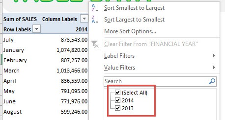
12. Show report filter on multiple pages

When you are using an Excel Pivot Table you can show the items within the Report Filter on separate sheets inside your workbook.

Say that you have created an awesome Pivot Table which shows total sales and number of transactions per region.

You can drop in your Customer field in the Report Filter and replicate the Pivot Table for each of your customers in a separate Sheet.

All you need to do is click inside your Table and in the menu ribbon under PivotTable Tools choose the Options tab and then select the Options drop-down and choose Show Report Filter Pages.

Each of your customers will have their unique Pivot Table in a separate Sheet with their individual sales and transactional metrics.

Here is our pivot table:

STEP 1: Drop the Customer Field in the report filter.

STEP 2: Go to Options > Options Drop Down > Show Report Filter Pages

STEP 3: Press OK.

Each customer’s table will show in a unique sheet!

13. Average

A Pivot Table is the most powerful feature within Excel as it allows you to analyze your data in many different ways, all with a press of a button.

The Summarize Values By option allows you to choose a type of calculation (Sum, Count, Average, Max, Min, Count Numbers Product, StdDev, StdDevp, Var, Varp) to summarize data from the selected field.

As a default when you drop in a values field in the Values area of the Pivot Table it will Sum it for you and give yo a Sum of Values.

You can change this calculation to an Average very easily, which will show you the Average values for your data.

STEP 1: Click in your data and go to Insert > Pivot Table

STEP 2: This will bring up the Create Pivot Table dialogue box and it will automatically select your data`s range or table.

In the Choose where you want the PivotTable report to be placed, you can either choose a New Worksheet or an Existing Worksheet.

If you choose a New Worksheet it will place the Pivot Table in a brand new worksheet (e.g. Sheet2).

If you decide to put the Pivot Table in an Existing Worksheet, you will need to select the location by pressing the red arrow, choosing the cell where you want your Pivot Table to be placed, and then pressing the ENTER key twice to confirm.

STEP 3: You will now need to drag and drop the Fields in the different areas of your Pivot Table

STEP 4: Now that your Pivot Table is set up, you need to Right Click in any of the Table values and choose Summarize Values By > Average

STEP 5: Now you have your Pivot Table report showing the Average Sales values per Region for each year:

14. Show a unique count

Excel 2013 added some new features to its arsenal and one that has been well overdue was the distinct or unique count.

Previously when we created a Pivot Table and dropped a customer field in the Row Labels and then again in the Values area we got the “total number of transactions” for each customer.

But what about if we want to show the total unique customers?

In Excel 2013 we can, by using the newly created Pivot Table Data Model:

STEP 1: Click in your data source and go to Insert > Pivot Table

STEP 2: The important step here is to “check” the Add this to the Data Model box and press OK

STEP 3: This will create a Pivot Table. Now drop the Customers field in the Row and Values areas which will give you the “total transactions” for each customer

STEP 4: To get a Distinct Count, you need to click on the Values drop-down for the Count of Customers and select the Value Field Settings

STEP 5: Under Summarize Values By tab, select the last option, Distinct Count and press OK

15. % of Grand Total

Excel Pivot Tables have a lot of useful calculations under the SHOW VALUES AS option and one that can help you a lot is the PERCENT OF GRAND TOTAL calculation.

This option will immediately calculate the percentages for you from a table filled with numbers such as sales data, expenses, attendance, or anything that can be quantified.

In the example below I show you how to get the Percent of Grand Total:

STEP 1: Insert a new Pivot table by clicking on your data and going to Insert > Pivot Table > New Worksheet or Existing Worksheet

STEP 2: In the ROWS section put in the Sales Month field, in the COLUMNS put in the Financial Year field and in the VALUES area you need to put in the Sales field twice, I explain why below:

STEP 3: Click the second Sales field’s (Sum of SALES2) drop down and choose Value Field Settings

STEP 4: Select the Show Values As tab and from the drop down choose % of Grand Total.

Also change the Custom Name into Percent of Grand Total to make it more presentable. Click OK.

STEP 5: Notice that the Percent of Grand Total data is in a decimal format that is hard to read:

To format the Percent of Grand Total column, click the second Sales field’s (Percent of Grand Total) drop down and choose Value Field Settings.

The goal here is for us to transform numbers from a decimal format (i.e. 0.23), into a percentage format that is more readable (i.e. 23%).

STEP 6: Click the Number Format button.

STEP 7: Inside the Format Cells dialog box, make your formatting changes within here and press OK twice.

In this example, we used the Percentage category to make our Percent of Grand Total numbers become more readable.

You now have your Table, showing the Percentage of Grand Total for the sales data of the years 2012, 2013, and 2014.

All of the sales numbers are now represented as a Percentage of the Grand Total of $32,064,332.00, which you can see on the lower right corner is represented as 100% in totality:

16. % of Column Total

Excel Pivot Tables have a lot of useful calculations under the SHOW VALUES AS option and one that can help you a lot is the PERCENT OF COLUMN TOTAL calculation.

This option will immediately calculate the percentages for you from a table filled with numbers such as sales data, expenses, attendance, or anything that can be quantified.

In the example below I show you how to get the Percent of Column Total:

STEP 1: Insert a new Pivot table by clicking on your data and going to Insert > Pivot Table > New Worksheet or Existing Worksheet

STEP 2: In the ROWS section put in the Sales Month field, in the COLUMNS put in the Financial Year field and in the VALUES area you need to put in the Sales field twice, I explain why below:

STEP 3: Click the second Sales field’s (Sum of SALES2) drop down and choose Value Field Settings

STEP 4: Select the Show Values As tab and from the drop-down choose % of Column Total.

Also, change the Custom Name into Percent of Column Total to make it more presentable. Click OK.

STEP 5: Notice that the Percent of Column Total data is in a decimal format that is hard to read:

To format the Percent of Column Total column, click the second Sales field’s (Percent of Column Total) drop down and choose Value Field Settings.

The goal here is for us to transform numbers from a decimal format (i.e. 0.23), into a percentage format that is more readable (i.e. 23%).

STEP 6: Click the Number Format button.

STEP 7: Inside the Format Cells dialog box, make your formatting changes within here and press OK twice.

In this example, we used the Percentage category to make our Percent of Column Total numbers become more readable.

You now have your Pivot Table, showing the Percent of Column Total for the sales data of years 2012, 2013, and 2014.

All of the sales numbers are now represented as a Percentage of each column (Years 2012, 2013 and 2014), which you can see on each column is represented as 100% in totality:

17. % of Row Total

Excel Pivot Tables have a lot of useful calculations under the SHOW VALUES AS option and one that can help you a lot is the PERCENT OF ROW TOTAL calculation.

This option will immediately calculate the percentages for you from a table filled with numbers such as sales data, expenses, attendance, or anything that can be quantified.

In the example below I show you how to get the Percent of Row Total:

STEP 1: Insert a new Pivot table by clicking on your data and going to Insert > Pivot Table > New Worksheet or Existing Worksheet

STEP 2: In the ROWS section put in the Sales Person field, in the COLUMNS put in the Financial Year field and in the VALUES area you need to put in the Sales field twice, I explain why below:

STEP 3: Click the second Sales field’s (Sum of SALES2) drop down and choose Value Field Settings

STEP 4: Select the Show Values As tab and from the drop-down choose % of Row Total.

Also, change the Custom Name into Percent of Row Total to make it more presentable. Click OK.

STEP 5: Notice that the Percent of Row Total data is in a decimal format that is hard to read:

To format the Percent of Row Total column, click the second Sales field’s (Percent of Row Total) drop down and choose Value Field Settings.

The goal here is for us to transform numbers from a decimal format (i.e. 0.23), into a percentage format that is more readable (i.e. 23%).

STEP 6: Click the Number Format button.

STEP 7: Inside the Format Cells dialog box, make your formatting changes within here and press OK twice.

In this example, we used the Percentage category to make our Percent of Row Total numbers become more readable.

You now have your Table, showing the Percent of Row Total for the sales data of years 2012, 2013, and 2014.

All of the sales numbers are now represented as a Percentage of each row (Years 2012, 2013, and 2014), which you can see on each row is represented as 100% in totality.

Particularly the yellow highlighted ones would total to 100% for the first row:

18. Difference From

Excel Pivot Tables have heaps of calculations under the SHOW VALUES AS option and one that gets the most use is the DIFFERENCE FROM calculation.

You can show the values as the Difference From previous months, years, day etc. This is just great when your boss asks you how you are tracking to the previous months, years, days…

In the example below I show you how to show the Difference From the previous YEAR:

STEP 1: Insert a Pivot Table by clicking on your data and going to Insert > Pivot Table > New Worksheet or Existing Worksheet

STEP 2: In the ROWS you have to put the Months field, in the COLUMNS the Years field and in the VALUES area the Sales field twice, I explain why below:

STEP 3: Now click on the second Sales field’s (Sum of SALES2) drop down and choose Value Field Settings

STEP 4: Now you need to select the Show Values As tab and from the drop-down choose the Difference From

STEP 5: You need to select the Base Item: (previous) and Base Field: Financial Year and press OK. So it will read the “Difference from the previous Financial Year”

STEP 6: To format the values you need to select the Table and go to Pivot Table Tools > Analyze/Options > Select > Entire Pivot Table.

Then you need to once again go to Pivot Table Tools > Analyze/Options > Select but this time select the Values

Now press CTRL+1 to bring up the Format Cells dialogue box and make your formatting changes within here and press OK.

NB: This will fix the number format permanently and any new field that gets added into the Pivot Table will have this format. Coll hey!

STEP 7: To change the Sum of SALES2 name within the Pivot Table, you need to click on a cell in the Pivot Table which contains the Sum of SALES2 and manually make the change and press Enter

STEP 8: You need to select the whole column that contains the empty values and Right Click and select Hide

You now have your Table, all formatted and showing the Difference from the previous Year:

19. Running Total in

A Running Total In is the accumulation of values over a certain period, like days, months, or years. It is sometimes referred to as the Year to Date analysis.

A Running Total In takes one period’s values, then adds a second period, then a third period…and so on, to give the accumulated values up to a certain period.

This can be shown in dollar form or in percentage form.

With an Excel Pivot Table, we can easily include this calculation without the need to use any formulas. Here is how:

STEP 1: Insert a Pivot Table by clicking in your data and going to Insert > Pivot Table and choose to insert it in a New or Existing Worksheet

STEP 2: You will need to put the Months Field in the ROW area, the Year Field in the COLUMN area and then put the Sales Field in the VALUES area two times!

STEP 3: Right Click on a Totals cell and choose Remove Grand Total

STEP 4: Right Click on a Sum of SALES2 value and select Show Values As > % Running Total In > Base Field: Month

STEP 5: You can manually change the name of the Sum of SALES2 Field by clicking in the cell’s title within the Pivot Table:

STEP 6: We can insert a Pivot Chart by clicking in our Pivot Table and going to PivotTable Tools > Analyze/Options > Pivot Chart

STEP 7: From the Insert Chart dialogue box you need to choose the Combo chart and “check”the Secondary Axis box for the YTD% Series and press OK

You now have your % Running Total In values on a Pivot Table and also shown graphically on a Pivot Chart:

20. Group by Date

Grouping Dates is very easy with a Pivot Table. All you have to do is Right Click on your Date values (which are either in the Row or Column Labels of your Table), then choose the Group option. From the dialogue box, you can choose to Group by Days, Months, Quarters, or Years.

STEP 1: Right-click on your Date values and choose Group.

STEP 2: Select the combination of grouping you prefer. Click OK.

Your pivot table is now grouped by dates!

21. Group by Quarters & Years

Ever encountered needing a quick report of total sales numbers by each quarter, of each year?

I was faced with this same scenario and looking at my data on hand, I only had sales numbers for each individual day.

Grouping these would take a ton of effort & complex formulas!

Thankfully there is the Pivot Table way, which is quick, easy, and reduces the risks of making any errors….and it makes updating the report easily with any new additional data!

In the example below I show you how to get the Sales Grouped by Quarters and Years:

STEP 1: Insert a new Pivot table by clicking on your data and going to Insert > Pivot Table > New Worksheet or Existing Worksheet

STEP 2: In the ROWS section put in the Order Date field.

Notice that in Excel 2016 (the version that I am using) it will automatically Group the Order Date into Years & Quarters:

STEP 3: If you do not have Excel 2016, right click on any Row value in your Pivot Table and select Group

STEP 4: In the Grouping dialogue box, Excel was able to determine our date range (minimum date and maximum date).

Make sure only Quarters and Years are selected (which will be highlighted in blue).

This will group our dates by the Quarters and Years. Click OK.

Notice that a Years field has been automatically added into our PivotTable Fields List. This is cool, as we can use this field for further Pivot Table analysis:

STEP 5: In the VALUES area put in the Sales field. This will get the total of the Sales for each Quarter-Year date range:

Now we have our sales numbers grouped by Years & Quarters!

Notice that we can improve the formatting:

STEP 6: Click the Sum of SALES and select Value Field Settings

STEP 7: Select Number Format

STEP 8: Select Currency. Click OK.

You now have your total sales for each quarterly period!

22. Sorting by Largest or Smallest

There are countless times when I had my Pivot Table all setup, but I was not really happy with how the data was sorted. The cool thing with Excel Pivot Tables, is it allows me to sort virtually anywhere!

Let us start off with this Excel Pivot Table showing the Sum of SALES for each Year and Quarter. Make sure to download the Excel Workbook below so that we will have the same starting point.

In the example below I show you how to Sort a Pivot Table by Largest or Smallest:

STEP 1: Right-click on a Year cell within the Pivot Table.

Go to Sort > Sort Newest to Oldest

This will sort our Years by descending order. Notice that 2014 was sorted first.

STEP 2: Now let us try to sort by Quarters.

Right click any Quarter name within the Pivot Table.

Go to Sort > Sort Newest to Oldest

This will sort our Quarters by descending order. Notice that Quarter 4 was sorted first.

STEP 3: Now let us try for the Sum of SALES.

Right-click on a sum value within the Pivot Table.

Go to Sort > Sort Largest to Smallest

This will sort our sum of Sales by descending order, regardless of the Quarter.

It’s pretty cool on how Pivot Tables Excel allow you to sort on any area that you want to!

23. Sort using a Custom List

A Custom List in Excel is very handy to fill a range of cells with your own personal list. It could be a list of your team members at work, countries, regions, phone numbers or customers.

The main goal of a custom list is to remove repetitive work and manual errors in inputting.

To demonstrate the power of Excel’s Custom Lists, we’ll explore what’s currently in Excel’s memory as a default list:

STEP 1: Type February in the first cell

STEP 2: From that first cell, click the lower right corner and drag it to the next 5 cells to the right

STEP 3: Release and you will see it get auto-populated to July (The succeeding months after February)

At first, it might seem like magic on how Excel does this!

Let us go straight into the Options in Excel to view how it’s being done, and how you can create your own Custom List:

STEP 4: Select the File tab

STEP 5: Click Options

STEP 6: Select the Advanced option

STEP 7: Scroll all the way down and under the General section, click Edit Custom Lists

Here you can see the built-in default Excel lists of the calendar months and the days.

If you click on a Custom List, you will see under List entries that it is greyed out and you cannot make any changes. This indicated that it is a default Excel Custom List.

STEP 8: You can create & add your own Custom List under the List entries section.

Click on NEW LIST under the Custom Lists area and then manually enter your list, entering one entry per line:

After typing the values, click Add.

In our screenshot below, we added the values of the Greek alphabet (alpha, beta, gamma, and so on)

Click OK once done.

STEP 9: Click OK again

STEP 10: Now let’s go back into our Excel workbook to see our new Custom List in action. Type alpha on a cell

STEP 11: From that cell, click the lower right corner and drag it to the next 5 cells to the right

STEP 12: Release and you will see it get auto-populated to zeta, which is based on our Custom List created in Step 8

 

24. Filter by Dates

There are an array of different Date filters in a Pivot Table. You can filter by a particular date range, for example: by this week, next month, next quarter, next year, last year, year to date and the list goes on and on. This is useful if you want to see what invoices are due to be paid this month or what sales transactions were included in a particular quarter.

Below I show you a few quick Pivot Table filter examples.

STEP 1: Go to Row Labels and select Date Filters > Between

STEP 2: Place a date range. Click OK.

Your pivot table is now filtered by the dates!

STEP 3: Let us try another one. Go to Row Labels and select Date Filters > Next Quarter

Your pivot table is now filtered by the next quarter!

25. Filter by Values – Top 5 Items

You can easily filter your Pivot Table to show your Top X customers. There are lots of different Value Filters to choose from and one of my favorites is the Top 10 Filter.

Here is our pivot table:

STEP 1: Go to Row Labels > Value Filters > Top 10

STEP 2: Set it to the Top 5 Items. Click OK.

Your pivot table is now filtered!

26. Insert a Slicer

Slicers in Excel are visual filters or interactive buttons that allow you to see what items have been chosen within a Pivot Table.

They are a new feature from Excel 2010 onward and Mac for Excel 2016 and a must for anyone wanting to wow their boss by adding interactivity in their reports! I show you how to insert a Pivot Table Slicer below:

STEP 1: Select your Pivot Table by clicking anywhere inside it.

STEP 2: Go to Options(Excel 2010)/Analyze(Excel 2013&2016) > Insert Slicer

Select the Month and Year Fields.

Click OK.

Your slicer is now ready! Go crazy clicking, slicing and dicing your data!

TIP: Hold down the CTRL key to select multiple items in your Slicer.

27. Slicer Styles

There are several different Slicer Styles available for you when you click on an Excel Slicer.

These Slicer Styles add color to your Excel workbook to gives it some much needed life!

You can also add columns to a Slicer and you can also find more Slicer options by Right Clicking on a Slicer.

I will show you how easy it is to choose the different Pivot Table Slicer Styles:

STEP 1: Select your Slicer.

STEP 2: Go to Slicer Tools > Options > Slicer Styles

Select a style you prefer by clicking on it with your mouse.

If you do not like the chosen Style, just follow the process above and choose another color!

Your Pivot Table Slicer now has come to life!

28. Slicer Connections for multiple pivot tables

Normally when you insert an Excel Slicer it is only connected to the Pivot Table that you are inserting it from.

What about if you had multiple Pivot Tables from the same data set and wanted to connect a Slicer to all of the Pivot Tables, so when you press a button all the Pivot Tables change?

Well this is possible with the Report Connections (Excel 2013 & 2016) / PivotTable Connections (Excel 2010) option within the Slicer. This is how it is achieved:

STEP 1: Create 2 Pivot Tables by clicking in your data set and selecting Insert > Pivot Table > New Worksheet/Existing Worksheet

Setup Pivot Table #1:

ROWS: Region

VALUES: Sum of Sales

Setup Pivot Table #2:

ROWS: Customer

VALUES: Sum of Sales

STEP 2: Click in Pivot Table #1 and insert a MONTH Slicer by going to PivotTable Tools > Analyze/Options > Insert Slicer > Month > OK

STEP 3: Click in Pivot Table #2 and insert a YEAR Slicer by going to PivotTable Tools > Analyze/Options > Insert Slicer > Year > OK

STEP 4: Right Click on Slicer #1 and go to Report Connections(Excel 2013 & 2016)/PivotTable Connections (Excel 2010) > “check” the PivotTable2 box and press OK

STEP 5: Right Click on Slicer #2 and go to Report Connections(Excel 2013)/PivotTable Connections (Excel 2010) > “check” the PivotTable1 box and press OK

Now as you select each Slicer’s items, both Pivot Tables Excel will change!

Have a look at the following image and the tutorial below that to see how this is achieved using Excel 2013:

29. Different ways to filter a Slicer

Excel Slicers are the best thing since sliced bread!

They are a new feature from Excel 2010 onward and Mac for Excel 2016 and are visual buttons that shows you what items have been filtered or selected in a Pivot Table.

There are several ways that you can filter an Excel Slicer. Download our workbook so you can practice:

LEFT MOUSE CLICK:

You can select items from the Slicer by using your left mouse button;

DRAG LEFT MOUSE BUTTON:

You can select an array of items by clicking the left mouse button and doing a dragging motion downwards/upwards within the Slicer;

CTRL KEYBOARD:

You can select multiple items by holding down the CTRL key on your keyboard and selecting the Slicer items with your left mouse button;

SHIFT KEYBOARD:

Select a Slicer item, hold down the SHIFT key on your keyboard and then select another Slicer item. This will select a range of items!

 

30. Creating a Calculated Field

Pivot Table Calculated Fields allow you to do mathematical calculations with your Field List. You can use any of the Excel mathematical equations, like /*+-%.

The only limitation is that you cannot reference any cells. Pivot Table Calculated Fields can be used to calculate percentage increases on Sales, margin calculations, or Cost of Goods sold, as I show below.

Here is our Pivot Table:

STEP 1: Click on the Pivot Table and Go to Options > Fields, Items, & Sets > Calculated Field

STEP 2: Set the Name to Cost of Goods Sold

STEP 3: Set the Formula to COSTS/SALES. This is the formula to be used for our calculated field.

STEP 4: The formatting is still not correct. Right click on the new column and select Number Format.

STEP 5: Select Percentage and click OK.

Your new calculated is now ready in percentage format!

31. Creating a Calculated Item

Pivot Table Calculated Items allow you to do mathematical calculations with your Item List. You can use any of the Excel mathematical equations, like /*+-%.

The only limitation is that you cannot reference any cells. Pivot Table Calculated Items can be used to calculate changes between each other, like a month´s or year’s value, averages or summation.

To activate the Calculated Item you have to make sure that you click on the chosen Item in the Pivot Table, then go to the PivotTable Tools tab in the Ribbon and go to Options > Fields, Items & Sets > Calculated Item.

STEP 1: Click on the item that you want to calculate.

STEP 2: Click on the Pivot Table and Go to Options > Fields, Items, & Sets > Calculated Item

STEP 3: Set the Name to Year on Year Variance

STEP 4: Set the Formula to use the Years: ‘2015’-‘2014’. Click OK.

Your Calculated Item is now ready!

32. Insert a Pivot Chart

Pivot Charts in Excel are an extension of a Pivot Table and they show its values in a graphical representation. So when you filter a Pivot Table, the Pivot Chart updates accordingly.

To insert a Pivot Chart you need to click in your Pivot Table, go to the PivotTable Tools tab in the Ribbon and choose Pivot Chart. Below I show you how easy this can be achieved and in a few clicks you can turn dull information in to colorful insight!

Here is our Pivot Table:

STEP 1: Click on your Pivot Table and go to Options > PivotChart

STEP 2: Select a Chart type and click OK.

You now have your cool Pivot Chart!

33. Pivot Chart & Slicers

Now we will take this concept once step further and insert a Slicer. The cool thing about this is that the Slicer will control both the Pivot Table and the Pivot Chart.

See how you can start creating some awesome interactive analytical reports in just a couple of steps.

Here we have our Pivot Table and Pivot Chart ready:

STEP 1: Click in your Pivot Table and go to Options > Insert Slicer

STEP 2: Select Region and Year. Click OK

You now have your Slicer and you can play around with it! It will affect both the Pivot Table and Pivot Chart!

34. Highlight Cell Rules based on values

A great way to highlight values within your data set, Excel Table or Pivot Table is to use Conditional Formatting rules.

Formatting cells that contain a specific criteria, for example, greater than X or less than X, is a good way to visualize your results.

When your criteria references a cell, then you can make this conditional format interactive. So as you manually change the referenced cell´s value, the conditional format gets updated and you can see the live results, as shown below….

STEP 1: Select a cell in your Pivot Table.

STEP 2: Go to Home > Conditional Formatting > New Rule

STEP 3: Set Apply Rule to the third option: All cells showing “Sum of SALES” values for “MONTH” and “YEAR”

STEP 4: Select a rule type: Format Only Cells That Contain

STEP 5: Edit the Rule Description. Go to Cell Value > Greater Than > Select The Cell

STEP 6: Select the cell format. Click Format and select a color. Click OK.

Try it out now! The highlight now happens dynamically when you update the value.

 

35. Directional Icons

Using a Pivot Table you can show the variance from your previous month’s sales very easily…

Now that we have the Pivot Table report above, we can show the variances per month using an up/down or directional icon suing Conditional Formatting.

STEP 1: Click on any variance value in the Pivot Table and go to Home > Conditional Formatting > Icon Sets > Directional

STEP 2: This will bring up the Apply Formatting Rule to dialogue box. Choose the 3rd option as this will apply the conditional format on all the values except the Subtotals

Your Pivot Table will look like this:

STEP 3: Now we need to make some edits in the Conditional Formatting Rule in order to get the Icons right.

Go to Home > Conditional Formatting > Manage Rules > Edit Rule

STEP 4: Inside the Edit Formatting Rule box you need to make the following changes:

Value = 0

Type = Number

“Check” the Show Icon Only box and press OK to confirm the changes:

STEP 5: In the next screen you will get the Conditional Formatting Rules Manager. Hit Apply to see the changes and OK to confirm them:

Now you have your Pivot Table showing the differences from the previous months with directional icons only!!!

36. Data Bars, Color Scales & Icon Sets

Conditional Formatting has improved in Excel 2010 with the introduction of Data Bars, Color Scales & Icon Sets.

Data Bars: Includes graphic bars in a cell, proportional to the cell’s value – Good for Financial Analysis

Color Scales: Includes a background color, proportional to the cell’s value – Good for Heat Maps

Icon Sets: Shows icons in a cell. The icons depend on the cell’s value – Good for Project Management reports

STEP 1: Select the range that you want to apply the conditional formatting on.

STEP 2: Go to Home > Conditional Formatting

STEP 3: It’s time to have fun! Select a Data Bar, Color Scale, or Icon Set and see what happens!

37. Intro to GETPIVOTDATA

What does it do?

A formula that extracts data stored in a Pivot Table

Formula breakdown:

=GETPIVOTDATA(data_field, pivot_table, [field1, item1], [field2,item2],…)

What it means:

=GETPIVOTDATA(return me this value from the Values Area, any cell within the Pivot Table, [and return me the value that pertains to this Field name, and this Field item],…)

---

The GETPIVOTDATA function in Excel returns data stored in a Pivot Table. So essentially it extracts the Pivot Table data to enable a user to create customized reports.

Think of the Pivot Table like your data source, so anything you see in the Pivot Table report can be extracted with the GETPIVOTDATA function and put into a cell within your worksheet.

The GETPIVOTDATA function becomes powerful when you reference cells to create shell reports, which you can see from the tutorial below.

NB. Only the Fields and Items that are included in the Pivot Table report (Row/Column Labels and Values area) can be used to extract their values.

STEP 1: We need to enter the GETPIVOTDATA function:

=GETPIVOTDATA(

STEP 2: The GETPIVOTDATA arguments:

data_field

What is the value that we want to return?

Type in SALES as we want to return the sales value:

=GETPIVOTDATA(“SALES”,

pivot_table

From which pivot table?

Just reference a cell in the pivot table, let’s type in $A$1

=GETPIVOTDATA(“SALES”, $A$1,

[field1, item1]

What are the fields that would serve as our filtering criteria?

To get our target sales figure, we will need: Sales Region, Financial Year, and Sales Quarter. To do this we will need 3 field-item pairs:

=GETPIVOTDATA(“SALES”, $A$1, “SALES REGION”, $A27, “FINANCIAL YEAR”, B$25, “SALES QTR”, B$26)

STEP 3: Do the same for the rest of the cells by copying the GETPIVOTDATA formula to the rest of the cells.

Now your new set of data is ready!

38. Refresh All for Pivot Tables

When the information in your data source gets updated or changed, you need to Refresh your Pivot Table to see those changes in your Pivot Table.

How about if you have multiple Pivot Tables from the same data source in the same workbook? Or;

Pivot Tables that are created from two different data sources in the same workbook?

In these scenarios, you can simply select Data > Refresh All and all your Pivot Tables will be updated automatically!

STEP 1: Change the information in your data set.

 

STEP 2: This is our Pivot Table. Take note of the cell that we expect to be updated:

 

Go to Data > Refresh All

 

The Pivot Table values are now updated with just a click!

39. Move an Excel Pivot Table

 

You have your Pivot Table ready, but it’s not in the best location. How can you move this?

In these scenario, you can simply select Move PivotTable and you can move an Excel Pivot Table easily!

For our example, let’s move this lovely Pivot Table upwards!

STEP 1: Make sure you have selected your Pivot Table. Go to Analyze > Actions > Move PivotTable

 

STEP 2: Select the new location where you want to move it. In our example, we selected cell A4. Click OK.

Voila! You have successfully moved your Pivot Table!

40. Show/Hide Field List of Excel Pivot Table

 

You have your Pivot Table ready, however all of a sudden your Field List is not showing up!

In these scenarios, you can simply Show / Hide Field List of Excel Pivot Table and you can bring back your Field List easily!

For our example, this is our Pivot Table:

STEP 1: To show the field list, right-click on your Pivot Table and select Show Field List.

Your Field List is now showing! Let us show in the next step how to hide this.

 

STEP 2: To hide the field list, right-click on your Pivot Table and select Hide Field List.

Your Field List is now hidden!

How to Show / Hide Field List in Excel

41. Pivot Table Styles

 

The default Pivot Table style in Excel is very bland and boring, stemming from a lack of creativity from the nerds over at Microsoft!

You can give some life to your Excel Pivot Table by simply changing the Pivot Table Style!

For our example, this is our Pivot Table:

STEP 1: Make sure you have your Pivot Table selected. Go to PivotTable Tools > Design > PivotTable Styles

 

STEP 2: Expand the styles list and have fun selecting your preferred style! You can see I selected the orange style below, as today is a hot day 🙂

You now have your Excel Pivot Table with your new warm style!

 

How to Change Pivot Table Styles in Excel

42. Sort manually

You have your Pivot Table ready, all sorted nicely both from a row and column perspective. However, you just need that one minor sorting tweak or two.

Well, Excel seemingly has a lot of tricks and you can even sort an Excel Pivot Table manually!

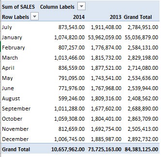
For our example, let’s see this Pivot Table below. It is sorted by years (2012-2014), and months (Jan-Dec).

But what if we want to move July to the top, and the year 2014 as the first column year?

STEP 1: To manually sort a row, click on the cell you want to move. Hover over the border of that cell until you see the four arrows:

 

Left mouse click, hold and drag it to the position you want (i.e. upwards to the first row)

We dragged it to the top so it’s now the first row!

 

STEP 2: To manually sort a column, click on the cell you want to move. Hover over the border of that cell until you see the four arrows.

Left mouse click, hold and drag it to the position you want (i.e. all the way to the left)

Voila! You have successfully manually sorted your Pivot Table!

 

EXTRA TIP: You can click inside a cell e.g. January, and start typing in another month, like August. This will also manually sort your Pivot Table items.

43. Use an External Data Source

When creating an Excel Pivot Table, what happens if your data source is in another location?

Would you have to copy your data into the same spreadsheet?

Well, NO! You can simply use the External Data Sources feature in your Pivot Table and Excel will magically import the data for you!

You can import data into your Pivot Table from the following data sources:

• Excel workbook
• Microsoft Access database
• SQL Server
• Analysis Services
• Windows Azure Marketplace
• OData Data Feed

 

For our example, we will import data using two data sources, an Excel workbook, and an Access file.

Import from another Excel Workbook:

Import From Microsoft Access and into Excel:

Wondering how this is even possible? Read on!

 

STEP 1: Go to Insert > Tables > PivotTable

 

STEP 2: Select Use an external data source and click Choose Connection.

 

STEP 3: Select Browse for More.

 

STEP 4: Select the Excel file with your data. Click Open.

 

STEP 5: Select the first option and click OK.

 

STEP 6: Click OK.

 

STEP 7: In the VALUES area put in the Sales field, for the COLUMNS area put in the Financial Year field, and for the ROWS area put in the Sales Month field

Your Pivot Table is ready from the Excel data source!

 

Import From Microsoft Access and into Excel:

 

STEP 1: Now let us try for an Access data source!

Go to Data > Get External Data > From Access

 

STEP 2: Select the Access Database Source file in your desktop or company file path. Click Open.

 

STEP 3: Select PivotTable Report and click OK.

 

STEP 4: In the VALUES area put in the Sales field, for the COLUMNS area put in the Financial Year field, and for the ROWS area put in the Sales Month field

Your Pivot Table is ready from the Access data source!

More Ways to Import External Data into an Excel Pivot Table:

You can also use this functionality to get data from other source types: SQL Server, Analysis Services, Windows Azure, and oData Data Feed

 

 

How to Use an External Data Source with Excel Pivot Tables

44. Clear and Delete Old Items

Have you ever cleared, deleted, or replaced your Pivot Table data/items but they still show inside your Pivot Table filters?

What gives??

Well, you can easily clear your Pivot Table’s old items from your Pivot Table’s memory or cache.

In our example below we have our Pivot Table with the Years showing in the Column area (2014, 2012, 2013):

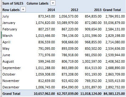
STEP 1: Below is our data source and we want to replace the year 2012 with 2013, effectively only showing the years 2014 & 2013.

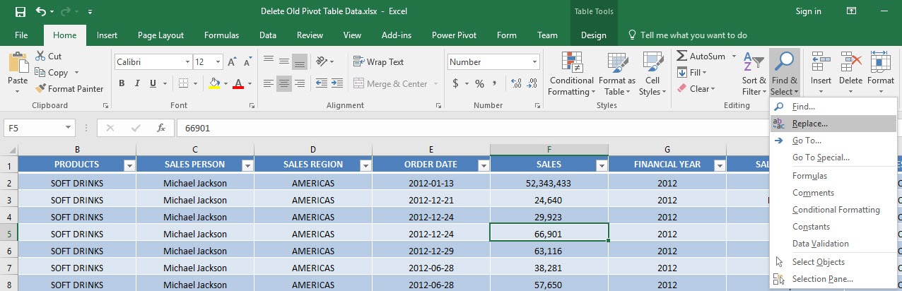
Go to Home > Find & Select > Replace

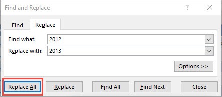
Let us replace the year 2012 with the year 2013. Click Replace All.

 

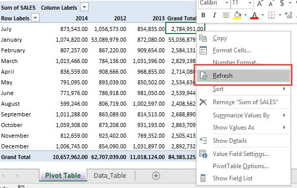
STEP 2: Go back to your Pivot Table. Right click and select Refresh.

 

We have technically deleted the year 2012 records, so they should be gone from our Pivot Table, right?

Hmm.. Looking good, the year 2012 is now gone from our Pivot Table!

 

BUT WAIT!

 

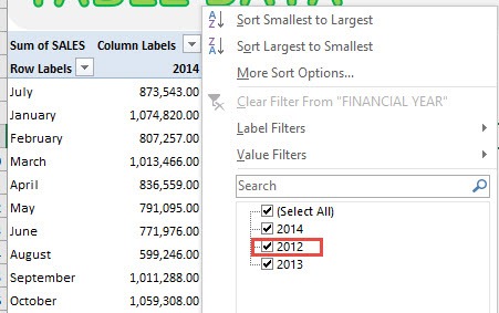
Clicking on the Column Labels drop-down list, the Year 2012 is still there! Bloody hell!

 

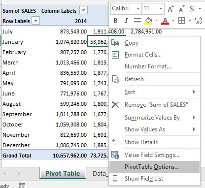
STEP 3: Let us fix this! Go back to your Pivot Table > Right-click and select PivotTable Options.

 

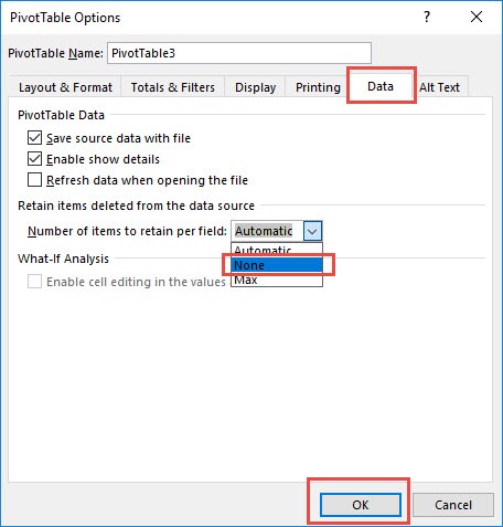
STEP 4: Go to Data > Number of items to retain per field.

Select None then OK. This will stop Excel from retaining deleted data!

 

STEP 5: Go back to your Pivot Table. Right-click and select Refresh.

 

Click the Column Labels drop-down list, and the Year 2012 is now gone! Problem fixed!

 

How To Clear & Delete Old Pivot Table Items

45. Count VS Sum

The #1 complaint that I get from Pivot Tables is “Why do my values show as a Count of rather than a Sumof ?”

Well, there are three reasons why this is the case:

1. There are blank cells in your values column within your data set; or

2. There are “text” cells in your values column within your data set; or

3. A Values field is Grouped within your Pivot Table.

 

1. BLANK CELL(S):

So if you have at least one blank cell in a Values column, Excel automatically thinks that the whole column is text-based. Pretty stupid but that’s the way it thinks.

2. TEXT CELL(S):

Also if you have a cell that is formatted as Text within your Values column, then it will also cause it to Count rather than Sum. This usually happens when you download data from your ERP or external system and it throws in numbers that are formatted as text e.g. 382821P

We get the annoying Count of Sales below:

Have a look at the following tutorials that show you how to locate blank cells: Find Blank Cells In Excel With A Color

EXCEL FIX:

STEP 1: You will need to enter a value or a zero within this blank or text formatted cell(s)

STEP 2: Go over to your Pivot Table, click on the Count of…. and drag it out of the Values area

STEP 3: Refresh your Pivot Table

STEP 4: Drop in the Values field (SALES) in the Values area once again

 

3. GROUPED VALUES:

Let’s say that you put a Values field (e.g. Sales) in the Row/Column Labels and then you Group it.

When you drop in the same Values field in the Values area, you will also get a Count of…

EXCEL FIX:

STEP 1: Right Click on the Grouped values in the Pivot Table and choose Ungroup:

STEP 2: Drag the Count of SALES out of the Values area and let go to remove it

STEP 3: Drop in the SALES field in the Values area once again

It will now show a Sum of SALES!

N.B. Sometimes you will need to locate the Pivot Table that has the Grouped values. The SALES field may not be evident that it is Grouped, especially if it is not selected in the Row/Column labels.

You may need to drag and drop this field from the PivotTable Fields and into the Row/Column Labels area to confirm that it is Grouped.

 

46. Automatically Refresh

Have you had challenges with constantly Refreshing a Pivot Table?

People forget that each time your data source gets updated that you will also need to manually Refresh your Pivot Table in order for it to get updated and show the changes made.

A lot of people ask if there is a way to automatically Refresh a Pivot Table, which I totally get. Automation is why we use Excel, right!

Here I show you a couple of ways that you can automatically Refresh a Pivot Table.

1. REFRESH PIVOT TABLE UPON OPENING:

This is a great feature and one that most people don’t know about.

It allows you to Refresh your Pivot Tables as soon as you open up your Excel workbook.

This is great if your Pivot Table’s data is linked to another workbook that gets updates by your colleagues and you only get to see the Pivot Table report.

 

STEP 1: Right Click in your Pivot Table and choose Pivot Table Options:

 

STEP 2: Select the Data tab and check the “Refresh data when opening the file” checkbox and OK

 

Now each morning that you open up your Excel workbook, you can be sure that the Pivot Table is refreshed!

 

2. AUTOMATIC REFRESH EVERY X MINUTES:

If you have your data set linked in an external data source, you can auto-refresh every x minutes.

Your data can be stored in an external data source such as Access, a Website, SQL Server, Azure Marketplace, etc.

STEP 1: If your data is stored externally, you will need to click in your Pivot Table and go to Properties (this will only be enabled for selection if you have an external data source)

 

STEP 2: This will open up the Connection Properties and you will need to select the Refresh every checkbox and manually set the time & press OK.

You can now sit back and enjoy a cup of coffee whilst your Pivot Table gets updated every few minutes:)

 

Automatically Refresh a Pivot Table

47. Frequency Distribution

With Excel Pivot Tables you can do a lot of stuff with your data! But did you know that you can even create a Frequency Distribution Table?

Let’s have some fun below! I’ll show you how easy it is to create your own Frequency Distribution Chart!

We will create a chart based on this table with Sales values:

 

STEP 1: Let us insert a new Pivot Table. Select your data and Go to Insert > Tables > PivotTable

 

Select Existing Worksheet and pick an empty space to place your Pivot Table. Click OK.

 

STEP 2: Drag SALES into VALUES and ROWS and you’ll see your Pivot Table get updated:

Click on Sum of SALES and select Value Field Settings.

Select Count and click OK.

 

STEP 3: We are almost there! Right click on your Pivot Table and select Group.

Accept the suggested values. It will group our values by ranges of 10,000. Click OK.

Now it’s grouped together!

 

STEP 4: Go to Analyze > Tools > PivotChart

Ensure Clustered Column is selected. Click OK.

Your awesome Frequency Distribution is now ready!

 

How to Create a Frequency Distribution

48. Slicer Connection Greyed Out

Sometimes when you create a Pivot Table and want to insert a Slicer you are unable to do this as the Slicer button is greyed.

You try to click on the Slicer button but nothing happens.

What gives??

There are two things that can cause your Slicer connection to be greyed out!

ONE: Your file format is in an older/incompatible format (e.g. a .xls file extension)

TWO: You can see the text [Compatibility Mode] right beside the name of your excel file:

Let me show you quickly how you can resolve this problem in just a few steps!

STEP 1: Go to File > Convert

 

STEP 2: This will convert your Excel file into a more updated version.

Click OK.

Click Yes to reload your workbook.

 

Voila! You can now insert your slicer!

NB: You can also Save As your current file as an .XLSX file format. Then close this file and open it again and you will be able to use the Slicer button again!

 

HOW TO ENABLE THE GREYED OUT SLIDER CONNECTION

Conclusion

In this tutorial, you have learned What is a Pivot Table in Excel and 50 different things you can do with an Excel Pivot Table.

Make sure to download our FREE PDF on the 333 Excel keyboard Shortcuts here:

*BONUS* FREE EXCEL PIVOT TABLE WEBINAR