How to Remove Character from String in Excel (Left or Right)

Microsoft Excel offers a suite of functions to clean up data, and removing unwanted characters is a common task that can be accomplished with ease. Understanding the right formulas, such as the LEFT, RIGHT, and SUBSTITUTE functions, unlocks the ability to streamline datasets by eliminating extraneous characters.

Key Takeaways

• Trimming text in Excel is crucial for data management to ensure clean and standardized data.
• Excel offers various functions like LEFT, RIGHT, SUBSTITUTE, and REPLACE for text manipulation, which help in parsing, extracting, and modifying strings.
• Flash Fill is a user-friendly feature in Excel that automatically detects patterns in data input and facilitates quick trimming.
• Excel’s advanced functions like SUBSTITUTE and REPLACE offer precision and control over text processing tasks, enabling users to remove character from string efficiently.

Download the spreadsheet and follow the blog on How to remove character from string in Excel – Download excel workbookRemove-Characters-from-String-in-Excel.xlsx

 

Strategies to Remove Character from String

Using the LEFT Function to Trim Text

The LEFT function in Excel is a versatile tool used for extracting a specified number of characters from the beginning of a text string. The syntax for the LEFT function is simple:

• text: The text string that you want to extract characters from.
• num_chars: The number of characters you wish to pull from the left side of the string.

For example, the formula =LEFT("apple", 3) returns "app" because it extracts the first three characters of the word “apple.

One use of this function is when you need to trim text by removing undesired characters from the left side. For instance, if you have product codes that always end with a certain number of useful characters, but vary in length at the beginning, you could use LEFT combined with the LEN function to remove unwanted prefixes:

Using the LEFT function is especially handy for cleaning up inconsistently formatted data and making it uniform for analysis and reporting. It allows Excel users to trim text confidently and accurately, which is fundamental in any data manipulation task.

 

Flash Fill as a Shortcut for Trimming

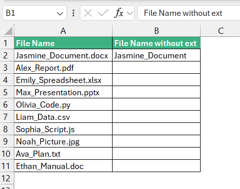
Flash Fill, introduced in Excel 2013, is like a smart assistant within Excel that intuitively recognizes patterns in your data input and automates text manipulation tasks accordingly. It offers a quick and user-friendly way to trim text without the need for complex formulas or functions.

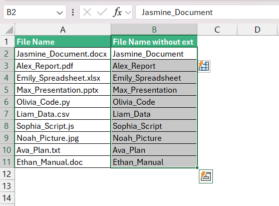
Suppose you have a column of text strings from which you want to remove unwanted characters at the beginning of each cell. With Flash Fill, you simply type the desired result in the cell adjacent to the original data and press Enter. Then, when you start typing the expected result in the next cell, Excel will detect the pattern and automatically suggest filling down the rest of the cells for you. If Excel’s guess at the pattern is correct, pressing the Enter key will accept the preview, and your data will be formatted in a flash.

Steps to use Flash Fill for trimming:

STEP 1: In a cell directly next to the one with the original data, enter the trimmed version of the text.

STEP 2: You can select the range where you need Flash Fill and use the keyboard shortcut Control + E (or Command + E on a Mac) to trigger it.

The beauty of Flash Fill lies in its simplicity and its capacity to discern a variety of patterns, from removing characters at the front or end of a string to more complicated extractions based on multiple delimiters.

A key tip when using Flash Fill for trimming is to provide a clear and consistent example(s) of the desired outcome in the initial cells. The more consistent the pattern, the more effective Flash Fill will be. Also, remember that Flash Fill operates based on text that you have already entered, making it an easy option for users who may not be comfortable with, or have time to learn, complex Excel functions.

 

Removing Characters from the Right with Speed

Harnessing RIGHT Function for Efficient Trimming

The RIGHT function in Excel is the counterpart to the LEFT function, designed specifically for extracting characters from the end of a text string. This function becomes incredibly useful when you need to trim characters from the right side—for instance, when dealing with data that has a consistent suffix you want to remove or when you need to isolate certain characters at the end of a string.

Here’s the basic syntax for the RIGHT function:

• text refers to the text string that you want to extract characters from.
• num_chars specifies the number of characters you want to pull from the right side of the string.

In a scenario where a text string in cell A2 contains “2023_Report.pdf” and you want just the file extension “pdf”, you could use the RIGHT function as follows:

This formula tells Excel to extract the last three characters of the string, on the assumption that all file extensions you’re dealing with are three characters long. If the number of characters to remove is dynamic, you would calculate it accordingly.

Utilizing the RIGHT function for efficient trimming is particularly beneficial for:

• Handling data with consistent formatting, such as strings ending with a specific set of characters (like file extensions or geographical codes).
• Processing information that includes unnecessary suffixes or padding for standardization before analysis.
• Preparing data for migrations between different systems that may require specific text formatting.

Remember, the RIGHT function processes data from the end of a text string, which is a crucial distinction from the LEFT function. Mastery of both these functions greatly enhances your Excel text manipulation toolkit and streamlines data management processes.

 

Advanced Tips for Quick Character Removal

Substitute Function

The SUBSTITUTE function can replace occurrences of a specified substring within a text string with new text. To remove a character, you can substitute it with an empty string (“”).

=SUBSTITUTE(text, old_text, new_text, [instance_num])

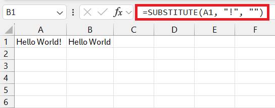
Let’s say you have the text string “Hello World!” in cell A1 and you want to remove the exclamation mark:

=SUBSTITUTE(A1, “!”, “”)

Replace Function

The REPLACE function replaces characters within a text string with new characters. To remove a character, you can replace it with an empty string (“”).

=REPLACE(old_text, start_num, num_chars, new_text)

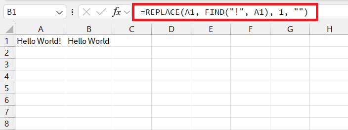
Let’s say you have the text string “Hello World!” in cell A1 and you want to remove the exclamation mark:

=REPLACE(A1, FIND(“!”, A1), 1, “”)

Here, FIND(“!”, A1) finds the position of the exclamation mark in the text string, and then REPLACE removes it by replacing 1 character starting from that position with an empty string.

These formulas will remove the specified character from the text string in cell A1. Adjust the character and cell references according to your specific requirements.

 

Batch Processing Text for Fast Adjustments

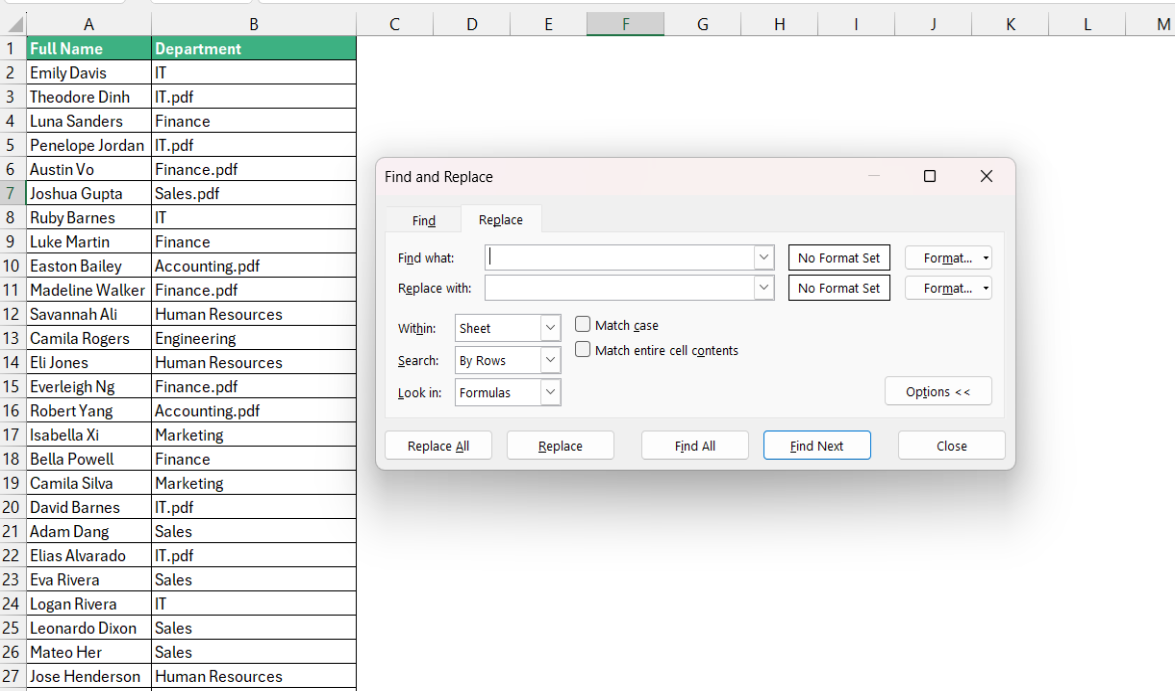
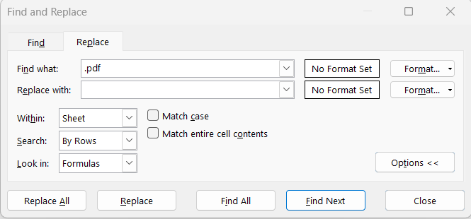
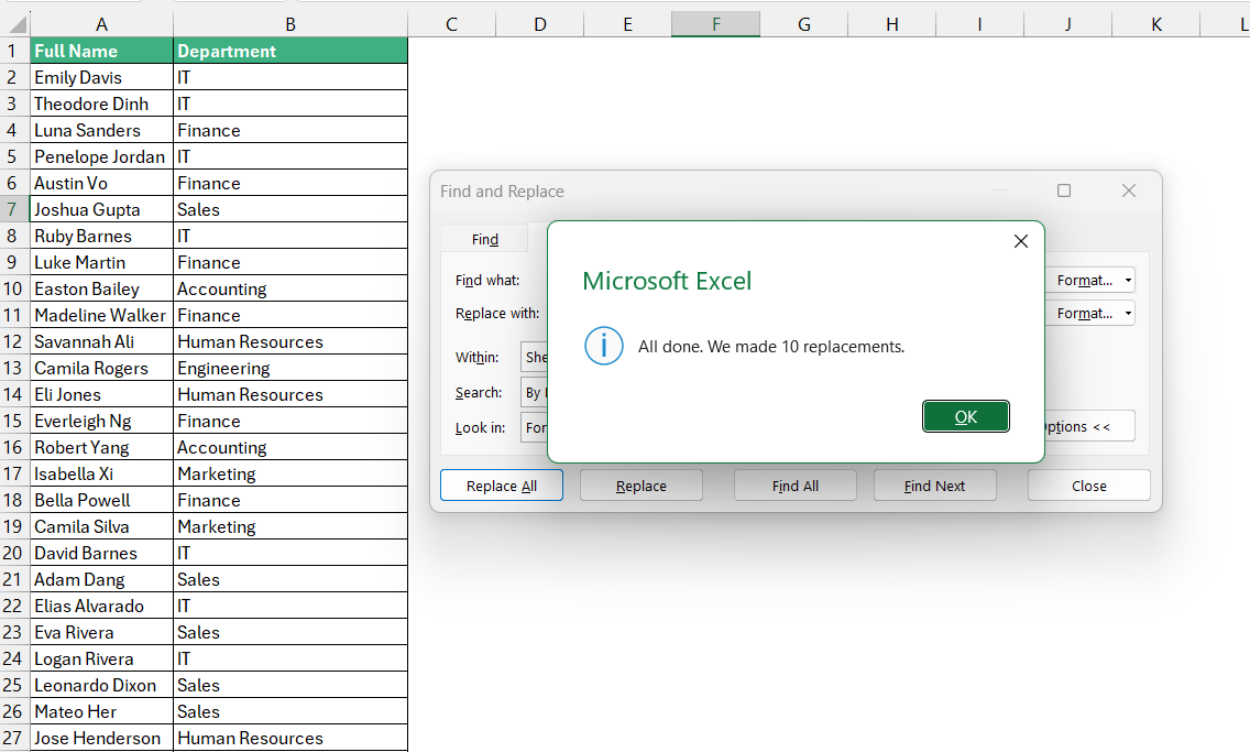
The Find and Replace feature (Ctrl+ H) is a handy tool for batch text adjustments. You can quickly search for a specific string or set of characters and replace them with an alternative or remove them entirely by replacing them with an empty string. This is particularly effective for removing characters or words from a dataset.

STEP 1: Press Ctrl + H to open the Find and Replace dialog.

STEP 2: Enter the text you wish to find in the “Find what” box and what you wish to replace it within the “Replace with” box (leave this blank to remove the text).

STEP 3: Select “Replace All” to make the changes throughout the entire selection or worksheet, or “Replace” to do it one by one.

 

 

FAQs

How can I remove only spaces from the text?

To remove only spaces from the text in Excel, use the TRIM function by selecting a cell adjacent to the text, typing the formula `=TRIM(A2)` if the text is in cell A2, and press Enter. This will trim extra spaces, and you can then apply this formula to the rest of the column by dragging the fill handle. If you’re looking to remove all instances of spaces including between words, instead use the Find and Replace feature by pressing Ctrl+H, entering a space in the “Find what” box, leaving the “Replace with” box empty, and clicking “Replace All.”

How do I remove certain characters from a string in Excel?

To remove specific characters from a string in Excel, you can use the SUBSTITUTE function with a formula like =SUBSTITUTE(B4, CHAR(202), “”) to target and remove unwanted characters. If you need to remove characters from the beginning or end of a string, you can use the =RIGHT(A2, LEN(A2) – 1) formula to remove the first character from the left, or the =LEFT(A2, LEN(A2) – 1) formula to remove the last character from the right. These formulas can be adjusted based on the position and number of characters you want to eliminate from your text strings.

How do I remove 3 characters from the left in Excel?

To remove three characters from the left of data in Excel, use the formula `=RIGHT(A1, LEN(A1) – 3)` in a nearby cell, where A1 is the cell containing the original data. Press Enter after typing the formula, and the resulting cell will display the content of A1 with the first three characters removed. If you need to apply this to multiple cells, drag the formula down using the fill handle to cover the desired range of cells.